Paper: Preventing Neural Network Weight Stealing via Network Obfuscation
Authors: Kalman Szentannai, Jalal Al-Afandi, and Andras Horvath
Venue: In Proceedings of the Computing Conference, 2020
URL: Preventing Neural Network Weight Stealing via Network Obfuscation
Introduction
In typical deep neural networks, small changes in weights do not cause significant changes in model predictions. From the perspective of model extraction attacks, this characteristic works in favor of the attacker. Attackers can replicate a well-trained original model, make minor modifications to the weights, and claim the model as their own. To address this issue, this paper proposes a method for creating a model that maintains the same accuracy as the original but is sensitive to even small weight changes.
Main Content
Fully Connected Layer
In deep learning, a Fully Connected Layer (FC Layer) is a linear transformation layer that connects every element of the input vector to every element of the output. In CNNs, after convolution layers learn local features such as edges, textures, and patterns within images, the FC Layer makes the final determination of which class the image belongs to based on these features.
This paper proposes a technique that modifies the structure of such FC Layers to introduce confusion into the network, creating a model where even small weight changes cause significant prediction changes.
Assuming three consecutively connected Fully Connected Layers, each layer is denoted as layer \(i-1, i, i+1\).
The method introduces confusion by modifying the middle layer \(i\) while keeping the end-to-end mapping from \(i-1\) to \(i+1\) unchanged. The middle layer \(i\) is modified by adding neurons. While the end-to-end mapping remains unchanged, the mappings between \(i-1\) and \(i\), and between \(i\) and \(i+1\), can be freely modified.
The output of layer \(i\) can be expressed by the following formula: \(x_i = \phi\!\left( W_{i_{N\times K}}\, x_{i-1} + b_i \right)\)
- \(N\) : Number of neurons in layer \(i-1\)
- \(K\) : Number of neurons in layer \(i\)
- \(W\) : Weights
- \(\phi\) : Activation function such as ReLU
- \(b_i\) : Bias of layer \(i\)
Based on this, the formula for \(i+1\) is expressed as follows: \(x_{i+1} = \phi\!\left( \phi\!\left( x\, W_{i-1_{N\times K}} + b_{i-1} \right)\, W_{i_{K\times L}} + b_i \right)\)
There are two main methods for adding neurons: decomposing neurons and adding deceptive neurons.
Decomposing Neurons
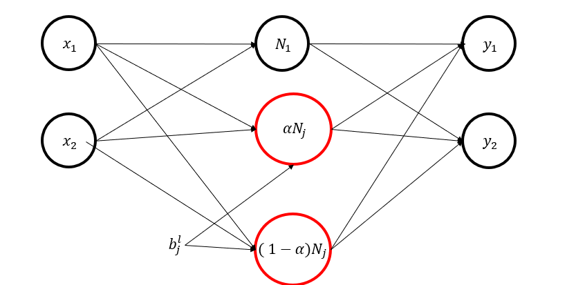
The first method decomposes an existing neuron into two neurons using an \(\alpha\) value between 0 and 1. The two neurons have the same bias as the original neuron and inherit the same weights connecting to the next layer. This way, the network’s overall input-output remains identical to before decomposition while the number of neurons increases.
\[\phi\!\Big(\sum_{i=1}^{n} W^{l}_{j i}\,x_i + b^{l}_{j}\Big) \;=\; N^{l}_{j}\] \[N^{l}_{j} \;=\; \alpha\,N^{l}_{j} \;+\; (1-\alpha)\,N^{l}_{j},\qquad \alpha\in(0,1)\]Here, \(\alpha\,N^{l}_{j}\) becomes the output of the first neuron after decomposition, and \((1-\alpha)N^{l}_{j}\) becomes the output of the second neuron.
This formula holds when the activation function is \(\phi(x) = max(0,x)\) and the activation switches must be the same, so the bias before and after decomposition must be identical.

After decomposing the two neurons, we need to determine the weights connecting the new neurons to the next layer. The simplest method is to use the same weights as before decomposition.
\[N^{l}_{j}\,\overline{W}^{\,l+1}_{j} \;=\; \alpha\,N^{l}_{j}\,\overline{W}^{\,l+1}_{j} \;+\; (1-\alpha)\,N^{l}_{j}\,\overline{W}^{\,l+1}_{j} \tag{7}\]This equation shows why weights can be reused as-is. The left side represents the influence of the original single neuron on the next layer before decomposition. The right side is the sum of the influences of the two new neurons on the next layer after decomposition. Since both values are exactly equal, it mathematically proves that decomposing a neuron into two causes no change in the network’s final result.
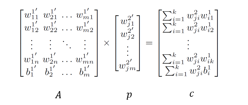
However, this simple method has the problem that an attacker can easily detect the structural modification of the network. To solve this, a system of linear equations \(Ap = c\) is used to set different weights for the new neurons. Through this process, the network’s internal connections (weights) change completely, but the overall function (output for a given input) remains perfectly identical.
-
\(p\): The unknown values we need to find. These are the new weight vectors used when connecting the decomposed neurons to the next layer.
-
\(A\): A matrix composed of already known values. It contains internal information of the decomposed neurons (input weights, bias, etc.).
-
\(c\): The target values we want to preserve. These represent the connection strengths (products of weights) that the original network possessed.
| According to linear algebra theory, the equation \(Ap = c\) has a solution only when rank(\(A\)) = rank([$$A | c$$]) is satisfied. (Rank refers to the rank of a matrix, i.e., the dimension of the vector space represented by the matrix.) |
The rule to always satisfy this condition is \(K \ge N + 1\).
- \(K\): Total number of new neurons in the layer after decomposition
- \(N\): Number of inputs the layer receives (e.g., number of neurons in the previous layer)
- +1: To account for the bias term
Deceptive Neurons
Simply decomposing neurons alone may allow an attacker to detect the manipulation by analyzing bias values, so a strategy of adding deceptive neurons is used to hide this. These deceptive neurons are designed to cancel each other’s effects so that their total sum is zero, having no impact on the network’s function. Mixing real and deceptive neurons into groups makes it exponentially difficult for an attacker to distinguish which are real and which are fake, making analysis practically impossible.
Deceptive neurons are always created in pairs to cancel each other’s effects. By creating pairs of real and deceptive neurons within groups that share the same bias, the neurons in the group appear similar to the attacker, making it difficult to distinguish between real and fake ones.
Experiment
The performance of the neuron decomposition method was first validated with a simple numerical setup.
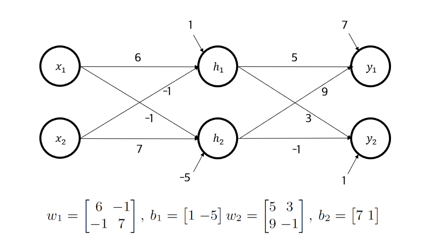
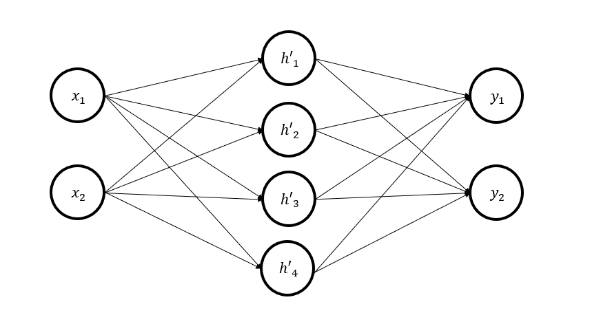
In the above structure, the middle layer neurons were decomposed into 4 neurons, and weights were found using the system of equations.
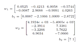
Then, the input vector was set to [7,9], and 1% noise was randomly injected into the weights to observe changes in output values.
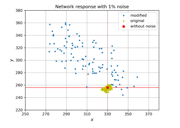
The graph shows that the output distribution when noise is added to the decomposed model is much wider than the output distribution when noise is added to the original model. This confirms that the technique of making the model’s output sensitive to weight changes through neuron decomposition was effectively applied.
Subsequently, additional experiments were conducted with a more complex structure. The experimental setup was as follows:
- Network architecture: 5 FC layers (input layer, 3 hidden layers, output layer)
- Number of neurons: 728, 32, 32, 32, 10 respectively
- Dataset: MNIST[8]
- Batch size: 32
- Optimizer: Adam
- Iterations: 7500
- Model test set accuracy after training: 98.4%
After training the model, additional neurons were created using the methods described above, with 9, 18, 36, and 72 neurons added in different experiments. The additional neurons were created equally across the 3 hidden layers, with 2/3 being deceptive neuron pairs and 1/3 being decomposed neurons. For example, when adding 36 neurons, each layer received 4x2 deceptive neuron pairs and 4 decomposed neurons.
After creating the modified models, noise was added to the weights in each case while measuring the model’s accuracy on the test set.
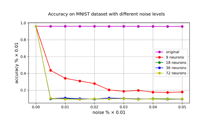
The graph shows that when no neurons are added, the model is robust to small noise. However, the modified models show a sharp drop in accuracy when a certain level of small noise is injected.
Subsequently, additional experiments were conducted to examine how sensitively accuracy responds to weight changes after further training the models with various optimizers (SGD, AdaGrad, Adam) and different step sizes. The results are as follows:
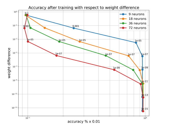
As expected, increasing the obfuscation level (adding more neurons) causes the model’s accuracy to drop significantly even with small noise.
Subsequently, experiments were conducted on the effectiveness of this defense technique when knowledge distillation, one of the attack methods, is applied. Knowledge distillation was performed by training a student model with 1 million random input samples.
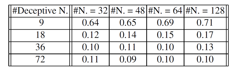
The columns of the graph represent the number of hidden layer neurons used by the attacker, and the rows represent the number of neurons added to the original model. The results show that when hidden neurons are 18 or more, the student model’s accuracy drops sharply to 10%-17%. This is similar to random guessing on the MNIST dataset (10 classes), effectively meaning complete failure in function replication. This experiment demonstrated that the proposed defense technique possesses very strong defensive capability against sophisticated model replication attacks such as knowledge distillation.
Conclusion
This paper presented a defense technique against model extraction attacks that create replicated models with small weight changes, by creating models that are sensitive to internal weight changes while maintaining original performance and function through adding extra neurons. The effectiveness of this approach was successfully demonstrated. This can be effective in protecting the intellectual property of network models and preventing unauthorized duplication and modification.