Paper: Perturbing Inputs to Prevent Model Stealing
Authors: Justin Grana
Venue: IEEE Conf. on Communications and Network Security, Avignon, France, 2020.
Introduction
Cloud-based machine learning services are typically provided as APIs that return predictions \(f(x)\) for input \(x\). Attackers repeatedly query such services to estimate model parameters or attempt to replicate the model. Existing defenses against such attacks are largely focused on post-processing outputs or post-hoc detection, including output rounding, noise injection, query request monitoring, and watermarking, which may become less effective when sufficiently many queries are made.
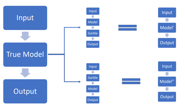
This paper proposes a method that garbles the input rather than the output, artificially creating endogeneity so that the attacker’s estimates do not converge to the true values even with infinite samples.
Background
Estimation Function \(h\)
The attacker estimates parameters \(\Theta\) based on collected data \((X,\hat{Y})\) through an estimation function h: \(\begin{align} h:X^N \times Y^N \to \Theta \end{align}\)
Attacker Estimators: OLS, MLE
The attacker attempts to estimate parameters through the following two methods:
- OLS (Ordinary Least Squares) minimizes the residual sum of squares \(\sum(\hat y_i-\alpha-\beta x_i)^2\) to obtain parameters \((\hat\alpha,\hat\beta)\).
- MLE (Maximum Likelihood Estimation) finds the parameters that maximize the likelihood or log-likelihood given the data. Under the Gaussian linear case, MLE becomes identical to OLS. In the logistic case, it maximizes \(\sum_i{y_i \log{p_i} + (1-y_i)\log{(1-p_i)}}\).
The key point is that input garbling creates correlation between variables and errors, causing both OLS and MLE to have asymptotic bias in large samples.
Evaluation Metrics
The following two metrics are used to evaluate defense performance:
- The attacker’s asymptotic estimation error is: \(\begin{align} D=\mathrm{plim}\,h(X,\hat Y)-\theta \end{align}\)
- The service’s prediction error is: \(\begin{align} \sigma^2=\mathbb{E}[(f_\theta(x)-f_\theta(g(x)))^2] \end{align}\) The goal is to keep \(D\) large and \(\sigma^2\) small.
Constraints
This paper applies the following constraint: \(\begin{align} \frac{1}{|X|}\sum\mathbb{E}[x-g(x)]=0 \end{align}\) This is a constraint to show that there is no net shift in the input on average. In practice, the proposed method works well even without this constraint, and the core results (bias and variance structure) are preserved.
Main Content
Simple Linear Regression: Large Sample Results (Prop. 1)
-
Large Sample In the simplest case, we define a linear machine learning model with a single variable as follows: \(\begin{align} f_{\theta}=\alpha+\beta x \end{align}\) The garbling function for the input is defined as: \(\begin{align} g(x)=x+\gamma(\mu(x,\lambda^2)) \end{align}\) Here, \(\mu(a,b)\) is a variable following the normal distribution \(\mathcal{N} (a,b)\).
Based on the above, the garbled prediction result \(\hat{y}\) is expressed as: \(\begin{align} \hat y=\alpha+\beta g(x) \end{align}\)
\[\begin{align} =\alpha+(1+\gamma)\beta x+\beta\gamma\lambda\varepsilon \quad \varepsilon \sim \mathcal{N}(0,1) \end{align}\]Therefore, the attacker’s estimation error \(D\) is: \(\begin{align} \mathrm{plim}\,\hat\beta=(1+\gamma)\beta \quad\Rightarrow\quad \,D=\beta\gamma \end{align}\) The service’s prediction error \(\sigma^2\) is: \(\begin{align} \sigma^2=(\beta\gamma)^2\{\mathrm{Var}(x)+\lambda^2\} \end{align}\) That is, in large samples, \(D\) is proportional only to \(\gamma\), while \(\sigma^2\) increases with both \(\gamma\) and \(\lambda\).
-
Small Sample (Finite Sample)
When the attacker attempts to estimate \(\beta\) via OLS or MLE with a finite number of queries, the following holds: \(\begin{align} \mathbb{E}[(\beta-\hat\beta)^2]=(\beta\gamma)^2+(\beta\gamma\lambda)^2\, \mathbb{E}\!\Big[\big(\sum_{i=1}^n x_i^2\big)^{-1}\Big] \end{align}\) That is, the larger \(\lambda\) is, the greater the error between the attacker’s estimated parameter \(\hat{\beta}\) and the actual parameter \(\beta\) in finite samples.
Therefore, in finite samples, a positive \(\lambda\) makes the attacker’s parameter extraction more difficult.
-
Identification Risk
The attacker can estimate the model’s parameters \(\hat{\alpha}\) and \(\hat{\beta}\), as well as the model’s variance \(\hat{\Sigma}^2 = \sum^N_{i=1}(\hat{y}-(\hat{\alpha}+\hat{\beta}x_i))^2\) through OLS or MLE. If the attacker knows \(\lambda\), the actual parameters can be recovered as follows: \(\begin{align} \hat{\Sigma}^2 \rightarrow (\beta\gamma\lambda)^2 \qquad(\hat{\Sigma}\to|\beta\gamma\lambda|) \end{align}\) \(\begin{align} \beta\gamma=\frac{\hat{\Sigma}}{\lambda},\qquad \hat\beta=\beta+\beta\gamma \ \Rightarrow\ \,\beta=\hat\beta-\frac{\hat{\Sigma}}{\lambda} \end{align}\) Therefore, \(\gamma,\lambda\) must be kept private and randomized.
Logistic Regression
The logistic regression model is as follows:
\[\begin{align} \hat y=\sigma\!\big(\alpha+\beta\,g(x)\big),\qquad \sigma(z)=\frac{1}{1+e^{-z}} \end{align}\]In the logit (linear score) space, the same relationship holds as in the linear case:
\[\begin{align} \mathrm{plim}\,\hat\beta=(1+\gamma)\beta \quad\Rightarrow\quad \,D=\beta\gamma \end{align}\]Meanwhile, in probability space, because the sigmoid function’s gradient is small in the tails, even as \(\gamma\) increases, the increase in probability error is gradual.
The following shows the visualization results of \(D\), \(\sigma^2\), and logit error as a function of \(\gamma\) in the logistic regression model:
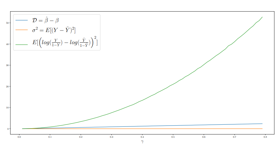
As \(\gamma\) increases, the logit error grows exponentially, and the estimation error (\(D\)) grows linearly, while the service’s prediction probability error (\(\sigma^2\)) increases gradually.
Multivariate and Multiple Garbling (Prop. 4)
Assume the following ML service: \(\begin{align} \hat{y} = f_{\theta} = \alpha + \beta_1 x_1 + \beta_2 x_2 \end{align}\) The following garbling is applied to each \(x_i\): \(\begin{align} g(x_i)=x_i+\gamma_i\,\mu_i(x_i,\lambda) \end{align}\)
Assume the attacker attempts to estimate parameters using OLS or MLE. The following relationships hold: \(\begin{align} \mathrm{plim}(\hat{\beta}_i)-\beta_i = \beta_i \gamma_i \end{align}\) \(\begin{align} \sigma^2 = [(\beta_1 \gamma_1)^2Var(x_1) + (\beta_2 \gamma_2)^2Var(x_2)+2\beta_1\beta_2\gamma_1\gamma_2\,\mathrm{Cov}(x_1,x_2)+(\lambda(\gamma_1 \beta_1 + \gamma_2 \beta_2))^2] \end{align}\) This shows that the scale of the bias is governed by \(\gamma_i\), as in the single-perturbation case, while the service prediction error is governed by the input covariance \(\Sigma\) and \(\lambda\).
Conclusion
This paper presents a defense that induces endogeneity through input garbling, causing the attacker’s parameter estimates to fail even with infinite samples. Defense performance is evaluated by the balance between the attacker’s estimation error \(D\) and the service’s prediction error \(\sigma^2\), and the key messages are as follows:
- Axis of inconsistency: \(\gamma\) creates asymptotic bias in the estimated parameters, which is independent of sample size. \(\lambda\) increases finite-sample variance, making replication difficult under initial or limited queries.
- Service loss management: \(\sigma^2\) is determined by the model, data distribution, and \(\gamma,\lambda\). In the linear case, \(\sigma^2\) decomposes into input covariance and \(\lambda^2\) terms. In the logistic case, low sensitivity in the sigmoid tails is exploited to produce large logit-space distortion while keeping probability-space loss small.
- Multivariate extension: Coordinate-wise garbling causes bias of \(\beta_i\gamma_i\) for each coefficient. While the input covariance \(\Sigma\) depends on external inputs, the defender can design the sign and magnitude of \(\gamma\) to achieve smaller \(\sigma^2\) for the same bias magnitude.
- Identification risk: If the attacker knows \(\lambda\), the actual parameters can be recovered from the residual standard deviation \(\hat\Sigma\) and \(\hat\beta\), so privacy and randomization of \(\gamma,\lambda\) are essential.
Scope and Limitations
The analysis is a proof of concept focused on linear and logistic models. Theory and empirical studies for large-scale nonlinear (DNN, etc.) models, dynamic interaction with attackers executing adaptive attacks (game-theoretic equilibrium), and tuning and monitoring procedures in operational environments remain as future work. Additionally, the premise is that the input distribution (and covariance) depends on external inputs, so the defender manages loss through garbling design tailored to the observed distribution rather than changing it.