Paper: Approximate Data Deletion from Machine Learning Models
Authors: Zachary Izzo, Mary Anne Smart, Kamalika Chaudhuri, and James Zou
Venue: International Conference on Artificial Intelligence and Statistics (AISTATS) 2020
Introduction
Deleting specific data from machine learning models is an important challenge for privacy protection and regulatory compliance. Regulations such as GDPR (General Data Protection Regulation) and CCPA (California Consumer Privacy Act) guarantee individuals the ‘Right to be Forgotten,’ allowing them to have their data deleted. However, even when data is deleted from a model, traces of that data may not completely disappear.
Existing methods required retraining the model from scratch to delete data. However, this is computationally expensive and inefficient. This paper proposes a new method called Projective Residual Update (PRU) that can efficiently delete data from linear regression and logistic regression models. PRU has linear computational complexity with respect to data dimensions and is independent of dataset size.
Additionally, “Approximate Data Deletion from Machine Learning Models” introduces a new metric called Feature Injection Test (FIT) to evaluate the effectiveness of data deletion, quantitatively measuring the efficacy of unlearning. This approach can improve efficiency in the data deletion process and more effectively support regulatory compliance for privacy protection.
Preliminary
This section explains the key notations and problem settings needed to understand Projective Residual Update (PRU) and Feature Injection Test (FIT).
Key Notation
-
\(n\): Total number of training data points
-
\(d\): Data dimension
-
\(k\): Number of data points to delete from the model
-
\(θ ∈ ℝ^d\): Model parameters
-
\(D^full = {(x_i, y_i)}_{i=1}^n ⊆ ℝ^d × ℝ\): Full training data set
-
\(X = [x_1 ... x_n]^T ∈ ℝ^(n×d)\): Full data matrix
-
\(Y = (y_1, ..., y_n)^T ∈ ℝ^n\): Response vector
Loss Function
The regularized loss function for the linear regression model is defined as follows.
\[\begin{equation} L^{\text{full}}(\theta) = \sum_{i=1}^n \ell(x_i, y_i; \theta) + \frac{\lambda}{2}\|\theta\|_2^2 \end{equation}\]Where
-
\(ℓ(x_i,y_i;θ)=12(θ⊤x_i−y_i)2\ell(x_i, y_i; \theta) = \frac{1}{2}(\theta^\top x_i - y_i)^2ℓ(x_i,y_i;θ)=21(θ⊤x_i−y_i)2\) is the ‘loss for a single data point.’
-
\(\lambda > 0\) represents the ‘regularization strength.’
The loss function excluding deleted data is expressed as follows.
\[\begin{equation} L^{\backslash k}(\theta) = \sum_{i=k+1}^n \ell(x_i, y_i; \theta) + \frac{\lambda}{2}\|\theta\|_2^2 \end{equation}\]Model Parameters
- \(\theta^{\text{full}} = \arg\min_\theta L^{\text{full}}(\theta)\) is the ‘model parameter trained on the full dataset.’
- \(\theta^{\backslash k} = \arg\min_\theta L^{\backslash k}(\theta)\) is the ‘model parameter excluding the deleted data.’
Main Content
This paper proposes a new method called Projective Residual Update (PRU) for efficiently deleting data from linear and logistic regression models, along with a new metric called Feature Injection Test (FIT).
Projective Residual Update (PRU)
Projective Residual Update (PRU) is an efficient algorithm that approximately computes model parameters excluding deletion-requested data.
Core Idea of PRU
- Compute residuals for the data points to be deleted.
- Update model parameters using the feature space of the data to be deleted.
- Compute the final parameters based on the modified residuals.
Core Formula of PRU
\[\begin{equation} \theta^{\text{res}} = \theta^{\text{full}} + proj_{\text{span}(x_1,...,x_k)}(\theta^{\backslash k} - \theta^{\text{full}}) \end{equation}\]Where \(\text{proj}_{\text{span}(x_1, \ldots, x_k)}(\cdot)\) is the ‘update operation based on the feature space of the data to be deleted.’
PRU Algorithm Description
To understand how PRU works, let us examine Algorithm 1 and Algorithm 2.
Algorithm 1: Projective Residual Update (PRU)
textprocedure PRU(X, Y, H, θ_full, k)
    # Step 1: Compute Leave-k-out predictions
    Ŷ_k ← LKO(X, Y, H, θ_full, k)

    # Step 2: Compute Pseudo-inverse
    S⁻¹ ← PseudoInv(∑_{i=1}^k x_i x_i^T)

    # Step 3: Compute Gradient
    ∇L ← ∑_{i=1}^k (θ_fullᵀ x_i - ŷ_k[i]) x_i

    # Step 4: Update parameters
    return θ_full - FastMult(S⁻¹, ∇L)
end procedure
The first algorithm is a method that updates parameters based on residuals, excluding specific data points, to maintain or improve the model’s performance.
The algorithm consists of the following steps.
First, in the Leave-k-out Predictions step, the model’s predictions are computed after excluding \(k\) samples from the dataset. This allows us to determine how much the model depends on specific data points. The predicted values \(Ŷ_k\) are based on the excluded data points and help evaluate how well the model generalizes.
Next, in the Pseudo-inverse Calculation step, the pseudo-inverse of the feature matrix is computed. The pseudo-inverse \(S^{-1}\) of the covariance matrix \(\sum_{i=1}^k x_i x_i^T\) of specific data points is obtained. This process accounts for linear dependencies in the data and provides the information needed for updating the model’s parameters.
Then, in the Gradient Calculation step, the gradient is computed based on the residuals. The residuals represent the difference between the model’s predicted values and the actual values, and \(\nabla L\) is obtained by multiplying these residuals by the weights of each data point and summing them. This gradient represents the current model’s performance and is used to determine the direction and magnitude of the parameter update.
Finally, in the Final Update step, the computed gradient is used to modify the existing parameters \(\theta^{\text{full}}\). This update is performed by multiplying the pseudo-inverse and the gradient, adjusting the parameters so that the model reduces the residuals. This step is a core process for improving the model’s performance.
Algorithm 2: Leave-k-out Predictions (LKO)
textprocedure LKO(X, Y, H, θ_full, k)
    # Step 1: Compute Residuals
    R ← Y_{1:k} - X_{1:k} θ_full

    # Step 2: Create Diagonal scaling matrix
    D ← diag({(1 - H_ii)⁻¹}_{i=1}^k)

    # Step 3: Create T matrix
    T_ij ← 1{i ≠ j} H_ij / (1 - H_jj)

    # Step 4: Compute final predictions
    Ŷ_k ← Y_{1:k} - (I - T)⁻¹ D R

    return Ŷ_k
end procedure
The second algorithm is a method for efficiently computing the values needed in Algorithm 1’s first step, focusing on obtaining prediction values after excluding specific data points.
The algorithm consists of the following steps.
First, residuals are computed by calculating the difference between the model’s predicted values and the actual values for the given data points. Residuals play an important role in evaluating how well the model is performing.
Next, a diagonal scaling matrix is created to adjust the importance of the residuals. This matrix reflects the importance of each data point and controls its influence on the model’s predictions.
Then, a T-matrix is created that reflects the correlations between remaining data points after excluding specific data points. This matrix provides information needed to adjust the prediction values.
Finally, the final prediction values are computed using the matrices created in the previous steps. This process adjusts predictions to maintain the model’s performance even after excluding data points.
Feature Injection Test (FIT)
Feature Injection Test (FIT) is a metric for evaluating how well sensitive features have been removed from a model.
A FIT score greater than 1 indicates that the feature still influences the model, while a score less than 1 indicates that the feature’s influence on the model’s predictions has decreased after deletion. This score is useful for quantitatively evaluating the effectiveness of data deletion and serves as an important metric for model safety and privacy protection.
FIT Measurement Process
- Feature Injection: Add a strong signal (feature) to specific data points.
- Model Training: Train the model using data that includes the injected feature.
- Post-deletion Evaluation: Verify whether the injected feature has been removed.
FIT Score Calculation \(\begin{equation} FIT = \frac{\text{Weight of injected feature (after deletion)}}{\text{Weight of injected feature (before deletion)}} \end{equation}\)
The weight of the injected feature (before deletion) is ‘the weight value when a specific feature has been injected into the model.’ This represents the influence that the feature has on the model’s predictions.
The weight of the injected feature (after deletion) is ‘the weight value after that feature has been deleted,’ evaluating the prediction performance after the feature has been removed from the model.
Comparison of Feature Injection Test (FIT) with Other Evaluation Metrics
Let us examine the differences between the existing evaluation metric $L^2$ distance and FIT.
\(L^2\) distance measures the overall parameter change but does not directly reflect whether sensitive features have been removed.
In contrast, Feature Injection Test (FIT) quantitatively measures how effectively sensitive features have been removed.
Experimental Results
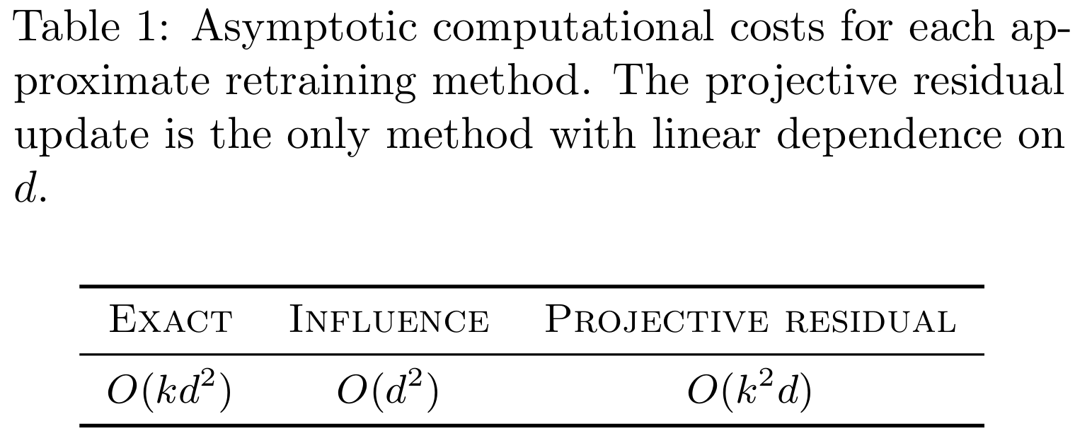
Table 1 shows that Projective Residual Update (PRU) has more efficient computational complexity than existing influence function-based methods. In particular, it confirms that PRU is more suitable for high-dimensional data.
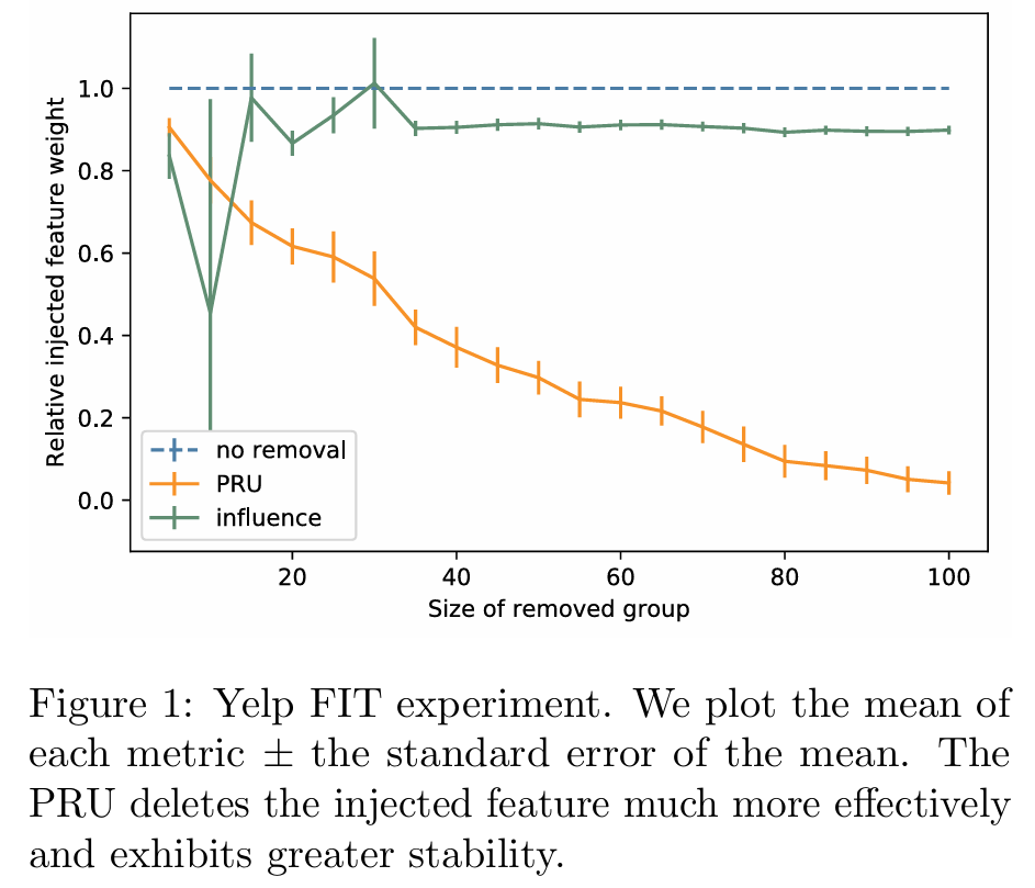
Figure 1 is a graph comparing FIT scores, showing that PRU removes injected features more stably and effectively.
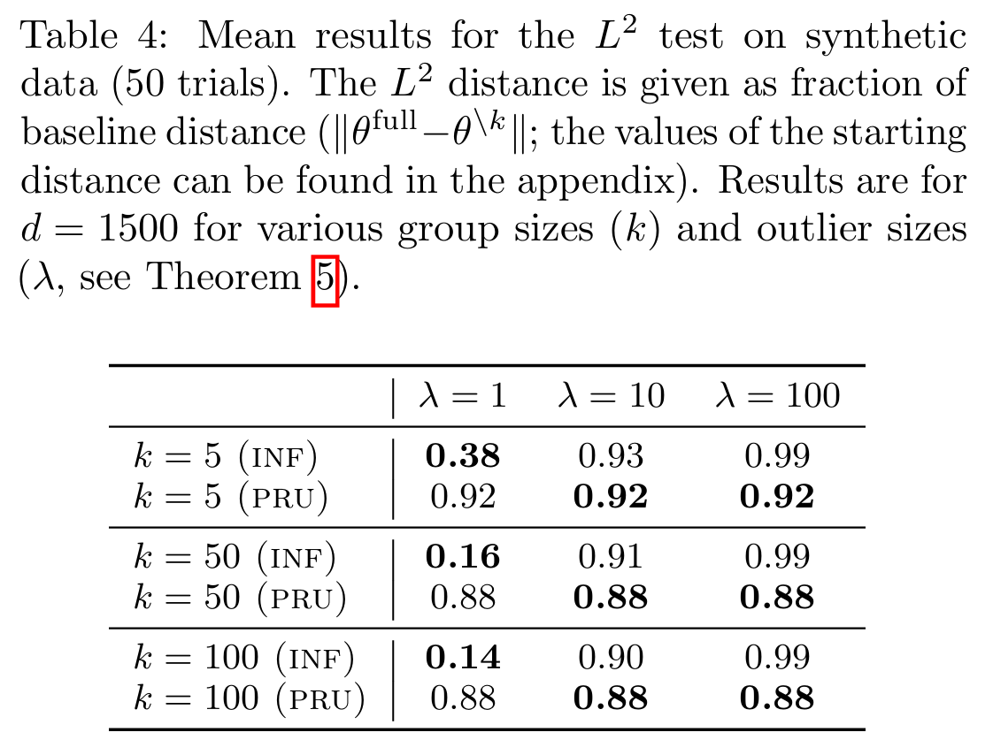
Table 4 shows that in sparse data environments, PRU is much more effective at completely removing sensitive features.
Conclusion
This paper proposes Projective Residual Update (PRU) and Feature Injection Test (FIT) for efficiently deleting data from linear and logistic regression models. PRU is faster and more accurate than existing methods, demonstrating excellent performance even on high-dimensional and large-scale datasets. FIT has been shown to be a tool that can quantitatively evaluate the ability to remove sensitive information, effectively measuring the effectiveness of data deletion.
These methods are expected to make significant contributions across various fields that must simultaneously consider privacy protection and model update efficiency. In particular, PRU enables real-time model updates on large-scale datasets, maintaining model accuracy even after data deletion.
Future research should focus on extending to nonlinear models and addressing the problem of processing continuous deletion requests. Such research will contribute to data management and privacy policy development.