Paper: Data-Free Model Extraction
Authors: Jean-Baptiste Truong, Robert J. Walls, Pratyush Maini, Nicolas Papernot
Venue: Proceedings of the IEEE/CVF conference on computer vision and pattern recognition, 2021
Introduction
Existing model extraction attacks are premised on the assumption that the attacker has access to a surrogate dataset similar to the victim model’s training data. However, in attacks targeting a truly black-box model, it is difficult to know what dataset was used during the model’s training phase.
This study proposes Data-Free Model Extraction, which does not require a surrogate dataset. That is, it presents a new approach that enables extracting the victim model without any separate training data.
Background
Knowledge Distillation
Knowledge Distillation is a knowledge transfer technique that trains a smaller-scale model (Student) to mimic the prediction information of an already trained large-scale model (Teacher).
It primarily uses a Teacher-Student structure, where the Student model takes the output distribution (soft labels) or logits obtained by querying the Teacher model as its learning objective.
Knowledge distillation is used to reduce the model’s scale while maintaining the accuracy of the large-scale model.
When performing knowledge distillation, since the model owner typically performs it, the Teacher model’s training dataset is often known. However, there are frequent cases where the dataset is too large or access to the dataset is impossible for security reasons. In such cases, Data-Free Knowledge Distillation (DFKD) is used.
Data-Free Knowledge Distillation (DFKD)
In situations where there is no access to the original data, to perform knowledge distillation, the Student model must create new input data to query the Teacher model.
In the DFKD technique, this role is performed by the input data generator (Generator).
The Generator is trained using the Teacher model’s output values, and the trained Generator produces input data optimized for the Student to query the Teacher.
Through this, the Teacher’s knowledge can be effectively transferred to the Student model without the original data.
The Data-Free Model Extraction presented in the main content draws inspiration from the DFKD mechanism described above and applies it to model extraction attacks.
Main Content
Data-Free Model Extraction
In Data-Free Model Extraction, leveraging knowledge distillation techniques, the target model (Victim) is set as the Teacher model, and the attacker’s extraction model is set as the Student model. The Generator then creates optimal queries so that the Student model can closely mimic the Victim model.
The Generator’s parameters are trained to produce optimal queries, and the Student model’s parameters are trained to produce outputs most similar to the Victim model’s for those queries.
Here, an optimal query is one that best reveals the discrepancy between the Victim model’s decision surface and the Student model’s decision surface. In simple terms, it means input data queries for which it is most difficult for the Student model to produce output matching the Victim model.
Therefore, the Generator is trained in the direction of maximizing the loss between the Victim model and the Student model.
Conversely, since the Student model’s goal is to create a model as similar to the Victim model as possible, it is trained in the direction of minimizing the loss.
The relationship between the Generator and Student model is similar to the relationship between the generator and discriminator in Generative Adversarial Networks (GANs).
The ultimate goal of Data-Free Model Extraction can be expressed as follows.
\[\arg\min_{\theta_S} \; \mathbb{P}_{x \sim \mathcal{D}_V} \left( \arg\max_i \mathcal{V}_i(x) \neq \arg\max_i \mathcal{S}_i(x) \right)\]- \(\mathcal{D}_V\): The input data domain used for training the Victim model
- \(\theta_S\): The parameter set of the Student model
- \(\mathbb{P}_{x \sim \mathcal{D}_V}\): The process of sampling \(x\) from the data pool \(\mathcal{D}_V\)
- \(\mathcal{V}_i(x)\): The Victim model’s probability (or logit) for class \(i\) given \(x\)
- \(\mathcal{S}_i(x)\): The Student model’s probability (or logit) for class \(i\) given \(x\)
- \(\arg\max_i\): Returns the class index with the highest value
The formula means optimizing the Student model’s parameters to minimize the prediction disagreement between the Student model and the Victim model for data sampled from the input data domain used for training the Victim model.
However, since this is a Data-Free model, access to \(\mathcal{D}_V\) is assumed to be unavailable. Therefore, synthetic input data created by the Generator is used. The reformulated model objective can be expressed as follows.
\[\arg\min_{\theta_S} \; \mathbb{E}_{x \sim \mathcal{D}_S} \left[ \mathcal{L}(\mathcal{V}(x), \mathcal{S}(x)) \right]\]- \(\mathcal{D}_S\): The synthesized dataset
- \(\mathbb{E}_{x \sim \mathcal{D}_S}\): The average of loss \(\mathcal{L}\) computed by sampling \(x\) from dataset \(\mathcal{D}_S\)
- \(\mathcal{L}(\mathcal{V}(x), \mathcal{S}(x))\): The loss function between the outputs of the Victim model \(\mathcal{V}\) and the Student model \(\mathcal{S}\)
The operation of Data-Free Model Extraction with this objective is shown in the figure.
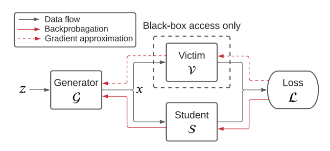
When random noise \(z \sim \mathcal{N}(0, 1)\) following a normal distribution enters the Generator as input, the Generator sends synthetic data queries to both the Student model and the Victim model.
The Student model then computes the loss for the difference with the Victim model’s output and learns its parameters through backpropagation in the direction of minimizing the loss.
The Generator is trained in the direction of maximizing that loss.
The model’s objective can be expressed as follows.
\[\min_{S} \max_{G} \; \mathbb{E}_{z \sim \mathcal{N}(0, 1)} \left[ \mathcal{L}(\mathcal{V}(\mathcal{G}(z)), \mathcal{S}(\mathcal{G}(z))) \right]\]The difference between the backpropagation processes of the Student model and the Generator is that while the Student model only needs its own output and the Victim model’s output for backpropagation, the Generator also requires the Victim model’s gradient. This is because the Generator learns its parameters to create queries that are most difficult for the Student model and Victim model to distinguish.
However, the gradient of the black-box Victim model is not disclosed. Therefore, a gradient approximation technique is needed to find the undisclosed Victim model’s gradient.
Black-box Gradient Approximation
Black-box Gradient Approximation is a technique for estimating gradients when actual gradients or internal parameters of a black-box model are inaccessible.
In particular, Zeroth Order Optimization methods can approximate gradients based solely on model output values.
In this process, a very small perturbation \(\epsilon\) is applied to the input \(x\), and the change in model output is observed to estimate the gradient. This can be expressed as follows.
\[\nabla f(x) \approx \frac{f(x + \epsilon) - f(x)}{\epsilon}\]Here, \(f(x)\) is the model’s output function, and \(\epsilon\) is a very small value.
The key idea of this method is to indirectly compute the gradient by slightly perturbing the input and comparing the resulting output changes when direct gradient access is unavailable in a black-box environment. The Victim model’s gradient is approximated in this manner.
Using multiple different \(\epsilon\) values results in a more accurate gradient approximation. Therefore, accuracy increases but the query complexity also increases proportionally, as more queries are required. Conversely, fewer \(\epsilon\) values reduce accuracy but also lower query complexity.
Therefore, finding an appropriate number of different \(\epsilon\) values is important.
Loss Function
A loss function must be defined to compute the difference between the Student model and the Victim model.
Traditionally, Kullback-Leibler (KL) Divergence is widely used. It is effective for aligning the Student model’s output distribution with the Victim model’s in knowledge distillation. The KL Divergence formula is as follows.
\[\mathcal{L}_{\mathrm{KL}}(x) = \sum_{i=1}^K \mathcal{V}_i(x) \log \left( \frac{\mathcal{V}_i(x)}{\mathcal{S}_i(x)} \right)\]Here, \(\mathcal{V}_i(x)\) and \(\mathcal{S}_i(x)\) are the probabilities predicted by the Victim and Student models for class \(i\), respectively. However, KL Divergence has the limitation of potentially suffering from vanishing gradient problems.
To overcome this limitation, L1 norm loss is also used. L1 loss directly computes the difference in logit values between the Victim and Student models, avoiding the vanishing gradient problem. The Victim’s logit values are assumed to be estimable from softmax output values.
The formula is as follows.
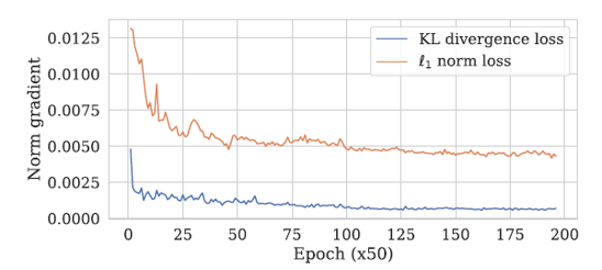
\[\mathcal{L}_{\ell_1}(x) = \sum_{i=1}^K \left| v_i - s_i \right|\]In practice, the magnitude of KL Loss’s gradient with respect to input \(x\) tends to become much smaller than L1 Loss’s gradient as the Student approaches the Victim. Therefore, L1 Loss can maintain training more stably, especially when the two models already make similar predictions.
Experiment
Algorithm
The algorithm for the experiments is shown in the following figure.
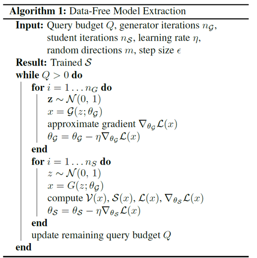
In this structure, the Generator \(G\) and Student \(S\) are trained alternately. In one iteration, the Generator is first trained for \(n_G\) steps, then the Student is trained for \(n_S\) steps.
-
Generator training phase (\(n_G\) iterations)
-
Sample \(z \sim \mathcal{N}(0, 1)\)
-
Generate \(x = G(z; \theta_G)\)
-
Compute loss
-
Approximate \(\nabla_{\theta_G} \mathcal{L}(x)\) using Gradient Approximation
-
Update the Generator to maximize the loss
\[\theta_G \leftarrow \theta_G + \eta \, \nabla_{\theta_G} \mathcal{L}(x)\]
-
-
Student training phase (\(n_S\) iterations)
-
Sample \(z \sim \mathcal{N}(0, 1)\)
-
Generate \(x = G(z; \theta_G)\)
-
Compute loss
-
Update the Student to minimize the loss
-
The training characteristics vary depending on the ratio of \(n_G\) and \(n_S\):
-
When \(n_G\) is high and \(n_S\) is low:
The Generator trains more and generates many difficult examples, but the Student may not be able to learn them sufficiently.
-
When \(n_G\) is low and \(n_S\) is high:
The Student trains extensively, but may lack learning on difficult examples.
Gradient Approximation in the Generator
In this study, gradient approximation is performed using the Forward Difference Method, expressed as follows.
\[\nabla_{\text{FWD}} f(x) = \frac{1}{m} \sum_{i=1}^m d \frac{f(x + \epsilon \mathbf{u}_i) - f(x)}{\epsilon} \mathbf{u}_i\]- \(\mathbf{u}_i\): Random direction vectors
- \(m\): Number of direction vectors \(\mathbf{u}_i\)
- \(\epsilon\): Small perturbation added
- \(f\): Loss function
As mentioned earlier, the number of queries changes according to the value of \(m\), which represents the number of random direction vectors, and accuracy and query count both increase as this value rises.
Experimental Setup
The experimental setup is as follows.
| Model | Architecture | Optimizer | Learning Rate | Epochs | Notes |
|---|---|---|---|---|---|
| Victim | (ResNet-34-8x) | SGD | 0.1 | 50 (SVHN) / 200 (CIFAR-10) | Query budget: 2M (SVHN), 20M (CIFAR-10) |
| Student | ResNet-16-8x | SGD | 0.1 | 50 (SVHN) / 200 (CIFAR-10) | - |
| Generator | 3 Conv + BatchNorm + ReLU | Adam | 5×10⁻⁴ | 50 (SVHN) / 200 (CIFAR-10) | Gradient approximation: m=1, ε=10⁻³ |
The Victim model used ResNet-34-8x and was trained on the SVHN and CIFAR-10 datasets with the settings described above.
Subsequently, the Student model and Generator were trained according to the algorithm described above.
Experimental Results
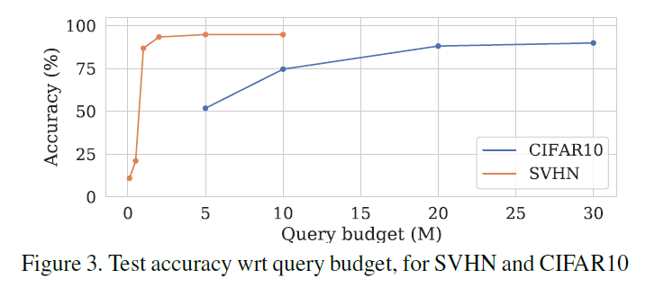
The graph above shows the experimental results of how the Student model changes as the query budget increases.
For the relatively simple SVHN dataset, optimal accuracy was reached and converged with approximately 2 million query budget, while for the more complex CIFAR-10 dataset, optimal accuracy was reached and converged with approximately 20 million query budget.
Ablation Study
After the experiments, ablation studies were conducted by varying the type of loss function and the values used in computing the loss function to examine their impact on Test Accuracy. The experimental results are as follows.
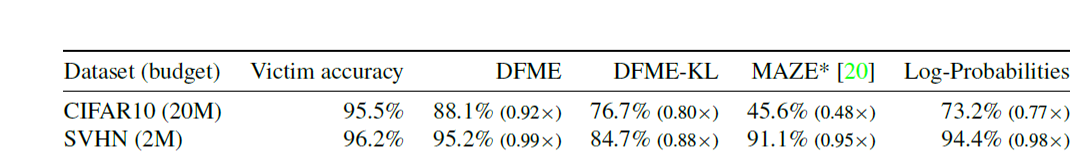
The values corresponding to each item in the table above are summarized as follows.
| Method | Loss Function | Values Used | Notes |
|---|---|---|---|
| DFME | L1 Loss | Logits | Proposed baseline method |
| DFME-KL | KL Loss | Logits | - |
| MAZE | - | - | Method proposed in another paper |
| Log-Probabilities | L1 Loss | Softmax | Uses the softmax output values directly without converting to logits |
The results show that optimal performance was achieved when using each model’s logit values as outputs and computing loss with L1 Loss.
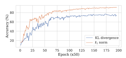
The results confirm that L1 Loss showed better performance than KL Divergence Loss.
The gradient vanishing problem was also more pronounced when using KL Divergence Loss compared to L1 Loss.
The next experiment examined how to best adjust the number of direction vectors \(m\) in the gradient approximation process.
Setting \(m\) to a large value increases the accuracy of gradient approximation, but also increases query complexity, causing a larger proportion of the total query budget to be used for generator training.
The query ratio ( r ) is calculated as follows:
\[r = \frac{n_S}{n_S + (m+1)n_G}\]-
\(n_G\): Number of generator training iterations
-
\(n_S\): Number of student model training iterations
-
\(m\): Number of random directions
For example, when \(n_G = 1\), \(n_S = 5\):
- If \(m = 1\), 71% of the query budget is used for student model training.
- If \(m = 10\), 31% of the query budget is used for student model training.
The remaining queries are used for generator training for better gradient estimation.
Experiments were conducted with different \(m\) values to find the optimal value. The results are shown in the following figures.
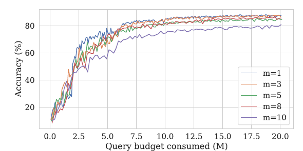
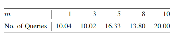
The graph above shows the accuracy change during model training for different \(m\) values, and the table shows the minimum number of queries needed for the model to first achieve 85% accuracy at different \(m\) values.
The table shows that lower \(m\) values allow reaching 85% accuracy faster with fewer queries.
When \(m = 1\), only a single random direction \(u\) is used to approximate the gradient. Even if the direction differs from the actual gradient vector’s direction, the gradient approximation process adjusts the sign to select either \(u\) or \(-u\), always aligning with the direction of increasing loss.
Therefore, in the early training phase when the Student model has not yet been trained, since the Student model cannot provide strong signals to the Generator, setting \(m = 1\) to focus on the Student’s initial training rather than Generator training, and then increasing the \(m\) value once the model has been trained to some degree, is the best approach for optimizing the model.
Conclusion
This paper demonstrated that Data-Free Model Extraction is feasible and that it can generate accurate replicas of the victim model. This implies that model extraction attacks can pose a serious threat to the intellectual property of publicly deployed models.
Additionally, as a future research direction, the paper suggests developing methods to detect such adversarial queries without degrading the model’s utility for normal users.