Paper: Practical Black-Box Attacks against Machine Learning
Authors: N. Papernot, P. McDaniel, I. Goodfellow, S. Jha, Z. B. Celik, and A. Swami
Venue: Proceedings of ACM ASIACCS, 2017
Introduction
Conventional adversarial example attacks have the limitation of relying on information about the model’s internal structure or training data. This paper overcomes these limitations and proposes an attack technique that works even in a black-box setting where such information is unknown.
In this paper, the attacker performs attacks against various models including DNNs under the assumption that only the model’s output labels can be observed. The attacker queries the original model to obtain labels, generates synthetic samples based on the Jacobian, and trains a substitute model. The paper then experimentally verifies whether adversarial examples generated using the substitute model transfer to the original model.
Experimental results showed a misclassification rate of 84.24% on MetaMind’s remote DNN, and 96.19% and 88.94% on Amazon and Google models, respectively. This demonstrates that a substitute model can effectively approximate the original model’s decision boundary through queries using only output labels.
Main Content
Substitute Model Training Process
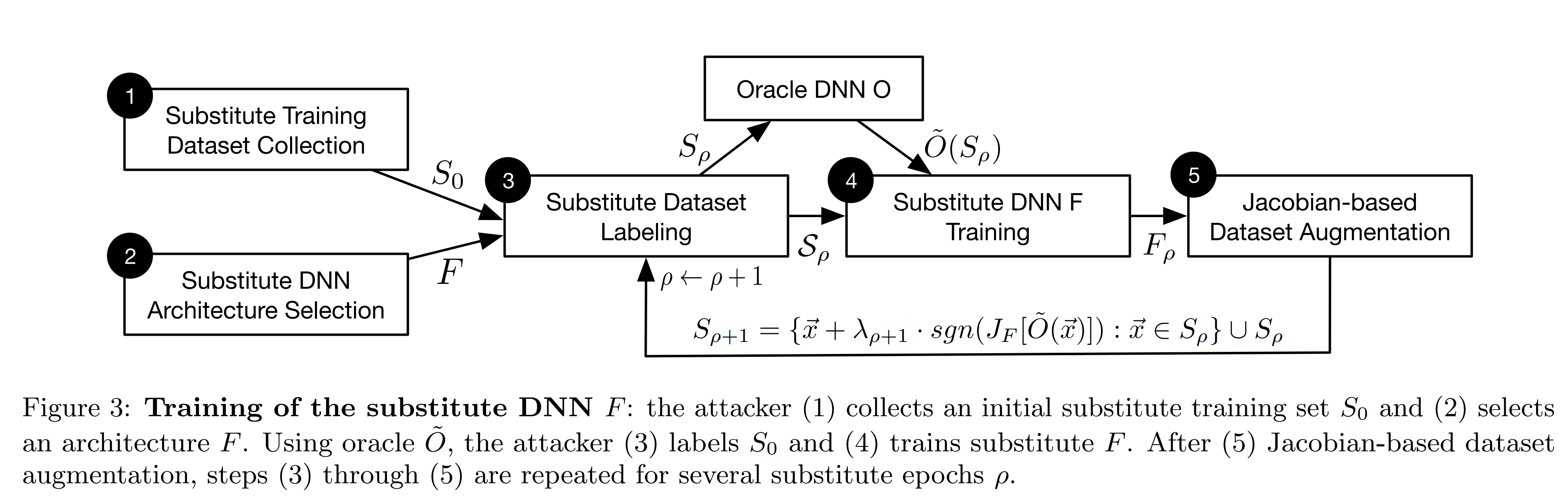
1. Initial Samples The attacker collects a small initial sample \(S_0\) representative of the input domain.
2. Substitute Model Architecture The attacker selects the architecture of the substitute model \(F\) based on the shape of the input and output data.
3. Dataset Creation The current training set \(S_\rho\) is input to the oracle \(O\) to obtain labels \(\tilde{O}(S_\rho)\). A dataset \(D\) is then created from the current training set and labels.
4. Substitute Model Training The substitute model is trained on the dataset to produce \(F_\rho\).
5. Synthetic Samples Synthetic samples are training data that help the substitute model better approximate the oracle’s decision boundary. The attacker computes the Jacobian matrix to determine in which direction the output of \(F\), trained using the oracle’s output results, changes most sensitively. The dataset is then modified along that direction to create synthetic samples, which are added to the previous training sample set \(S_\rho\) to form \(S_{\rho+1}\). The process then repeats from step 3.
After iterating steps 3-5 to retrain the substitute model, the attacker uses the substitute model to craft adversarial examples for the attack. In this paper, they are crafted using FGSM and the Papernot algorithm.
FGSM
FGSM (Fast Gradient Sign Method) modifies input data by following the sign of the gradient of the cost function with respect to the input direction.
\[\vec{x}^{*}=\vec{x}+\delta_{\vec{x}}\] \[\vec{x}^{*}=\vec{x}+\varepsilon\,\operatorname{sgn}\!\big(\nabla_{\vec{x}}c(F,\vec{x},y)\big)\]FGSM can quickly modify input data, and the modified data serves as adversarial examples that induce model misclassification. Increasing epsilon raises the likelihood of misclassification, but also makes changes more perceptible to the human eye.
Papernot Algorithm
The Papernot algorithm differs from the conventional FGSM approach. FGSM modifies all components of the input data by the same magnitude, designed to avoid classification into the correct class. However, this limits its ability to induce misclassification into a specific class.
In contrast, the Papernot algorithm selectively modifies only some components of the input data, making it suitable for misclassifying samples of all classes into an arbitrary target class t. To this end, it determines the whether to modify each component based on the saliency value of each input component. When the target misclassification class is t, the saliency value for the \(i\)-th component is calculated by the following formula:
\[S(\vec{x}, t)[i]= \begin{cases} 0 \ \ \ \ \ \text{if} \ \ \displaystyle \frac{\partial F_t}{\partial \vec{x}_i}(\vec{x})<0 \ \text{or}\ \displaystyle\sum_{j\ne t}\frac{\partial F_j}{\partial \vec{x}_i}(\vec{x})>0\\[10pt] \displaystyle \frac{\partial F_t}{\partial \vec{x}_i}(\vec{x})\,\left|\sum_{j\ne t}\frac{\partial F_j}{\partial \vec{x}_i}(\vec{x})\right| \ \ \ \ \ \ \ \ \ \ \ \ \text{otherwise} \end{cases}\]Input components with a saliency value of 0 are excluded from modification. This applies when increasing a specific input component decreases the output toward target class t, or increases the output toward non-target class j.
Conversely, when increasing a specific input component increases the output toward target class t, or decreases the output toward non-target class j, the saliency value is determined by its magnitude.
The higher the saliency value of an input component, the greater the likelihood of misclassification into target class t when modified. Therefore, saliency values are sorted in descending order, and components are modified sequentially starting from the highest value to generate adversarial examples. The modification magnitude \(\delta_{\vec{x}}\) applied to each selected component is set to \(\varepsilon\) in the subsequent experiments.
\[\vec{x}^{*}=\vec{x}+\delta_{\vec{x}}\]Experiments
Experimental Setup
Experiments were conducted on MNIST data, using MetaMind’s DNN API as the oracle.
Substitute Model Classification Performance
This paper is based on the premise that the attacker cannot access the oracle’s training data. Therefore, the attacker must verify that a substitute model trained on handwritten data performs similarly to one trained on actual training data. To verify this, 100 handwritten digit images and 150 MNIST test set images were each used as initial training samples for a DNN substitute model, and performance was compared.
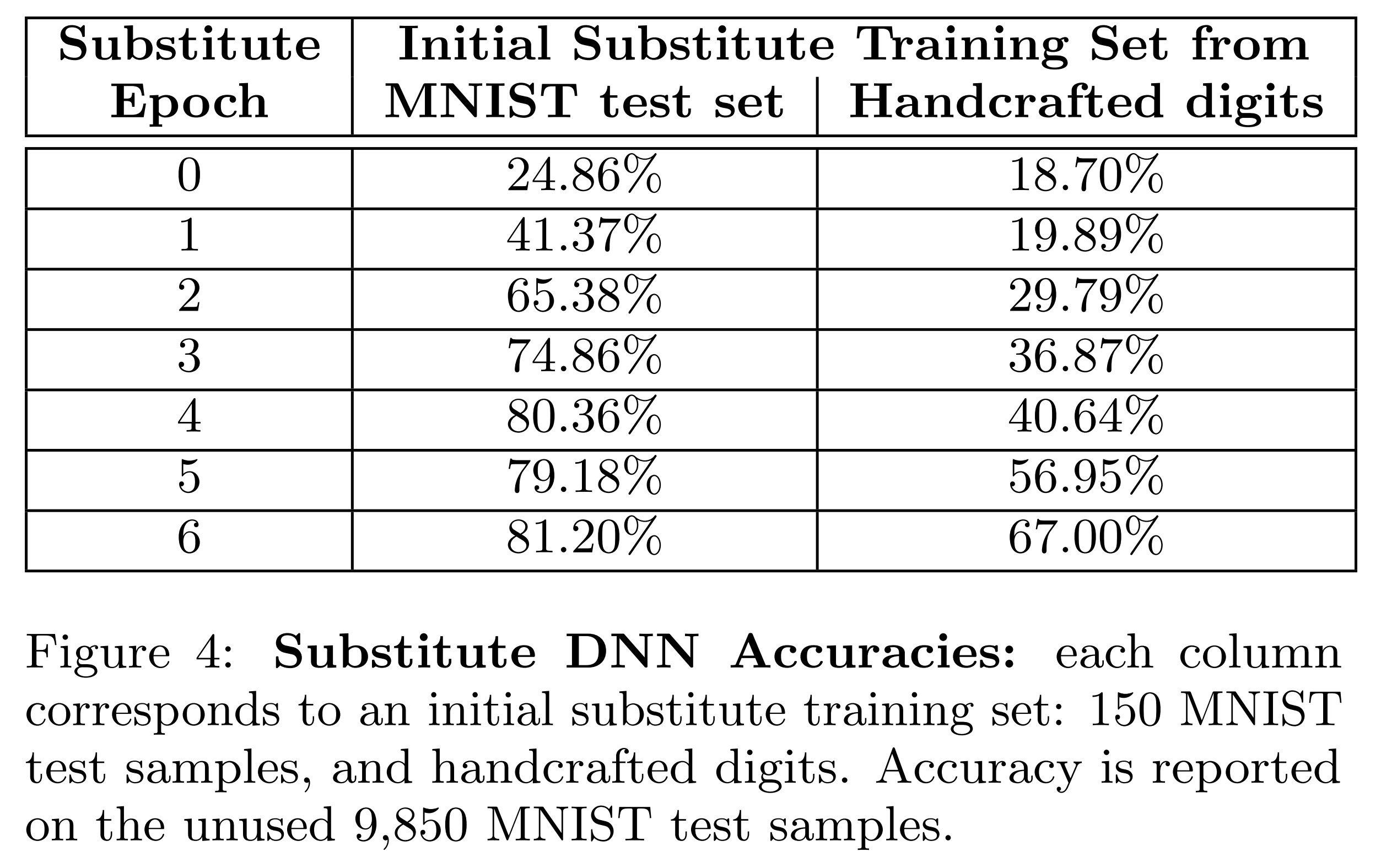
The above results show the accuracy when inputting the MNIST test set to each substitute model. The accuracy with handwritten data was 67%, lower than when using MNIST training data.
However, the main goal of this experiment is not to increase the substitute model’s accuracy, but to verify whether the substitute model effectively approximates the original model’s decision boundary. Verification of this continues in the next experiment.
Decision Boundary Approximation Performance of Substitute Models
For the two substitute models used in the above experiment, adversarial examples are generated using FGSM. These are then input to both the substitute model and the original model to check misclassification success. The performance variation with FGSM’s epsilon size is also examined.
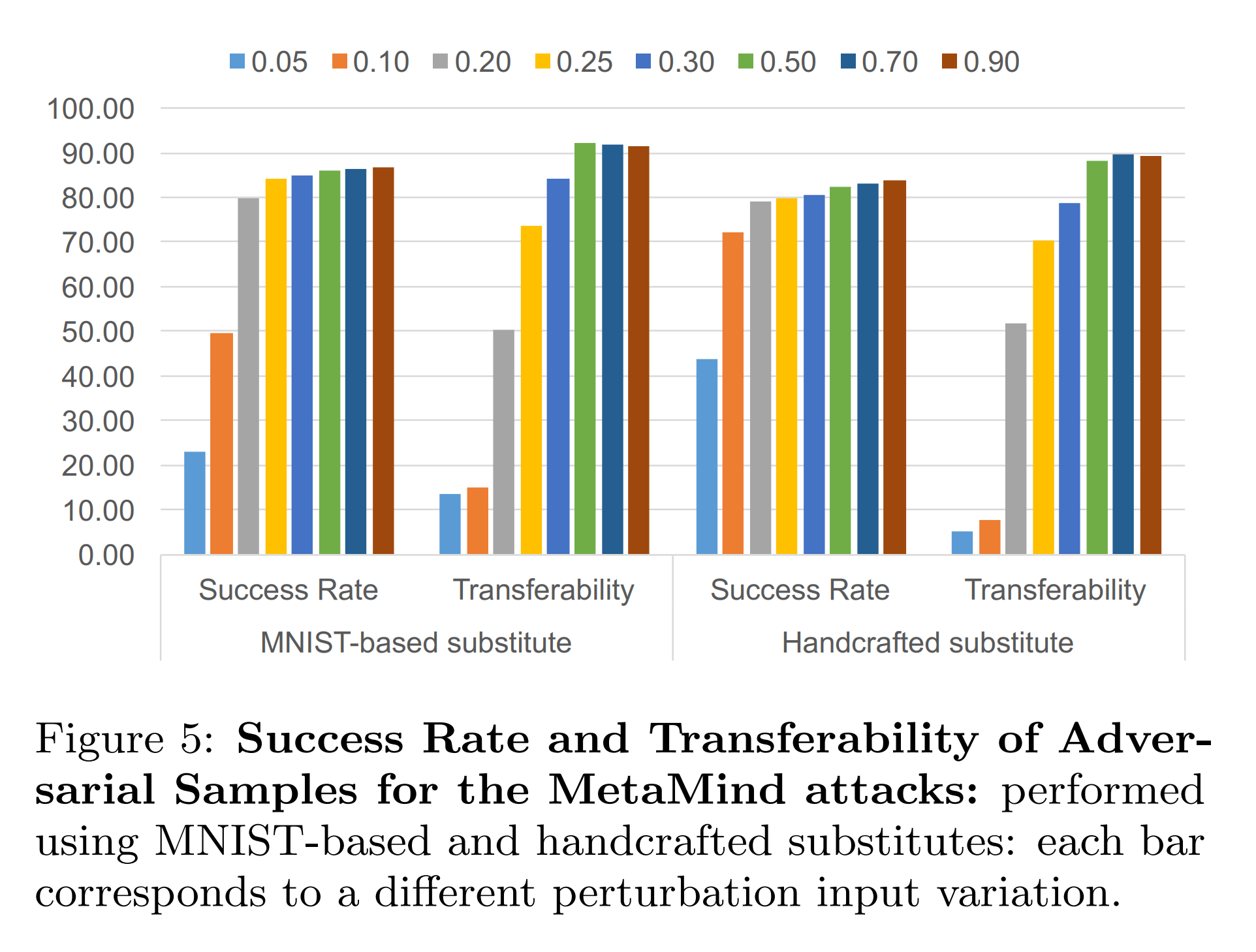
- Success Rate: The proportion of adversarial examples misclassified by the substitute model
- Transferability: The proportion of the same adversarial examples misclassified by the original model
The results show that both substitute models exhibited similar transferability. This suggests that the attack is feasible even when the attacker cannot access the oracle’s training data.
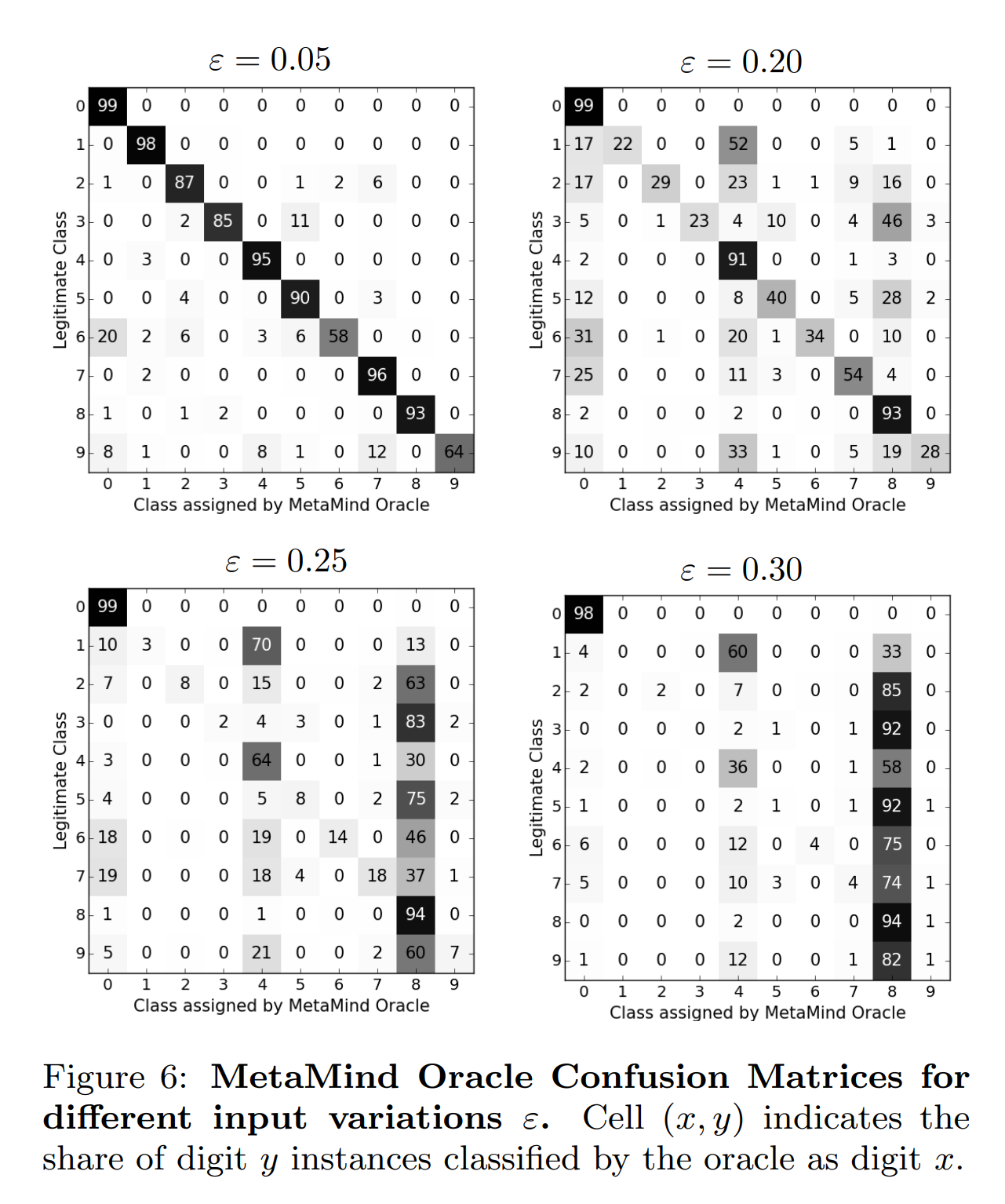
Additionally, the experimental results below show the outcomes of inputting adversarial examples crafted from the substitute model to the original model. Diagonal elements represent correct classifications by the original model, and off-diagonal elements represent misclassifications. As a result, as epsilon increases, the classes misclassified by the original model tend to converge consistently.
Calibration Experiments
Objective
Identify which parameters in the DNN substitute model training process and adversarial example crafting process can be adjusted to improve the substitute model’s performance.
Substitute Model Training Characteristics
-
Substitute Model Architecture The choice of model architecture such as number of layers, size, activation function, and type had little impact on transferability.
-
Number of Epochs Once the substitute model’s accuracy reached saturation, increasing epochs further did not improve transferability.
-
Step Size lambda When adjusting the lambda used to create synthetic samples for substitute model training, accuracy change was within plus or minus 3% from the baseline of 0.1. Increasing lambda degraded convergence stability, while decreasing it slowed convergence speed.
Additionally, as shown in the results below, transferability of the substitute model decreased as lambda increased.
lambda = 0.1 lambda = 0.3 epsilon = 0.25 22.35% 10.82% epsilon = 0.5 85.22% 82.07%
Substitute Model Training Improvements
-
PSS Synthetic samples are added each round according to the following formula:
\[S_{\rho+1}=\{\;\vec{x}+\lambda_{\rho+1}\cdot \operatorname{sgn}\!\big(J_{F}[\tilde{O}(\vec{x})]\big)\;:\;\vec{x}\in S_{\rho}\;\}\cup S_{\rho}\]During repeated retraining, if synthetic samples keep being modified in the same sign direction, they eventually go outside the input range ([0,1]). Clipping to the valid range is needed to address this, but repeated clipping causes synthetic samples to concentrate in specific regions. As a result, the substitute model struggles to precisely explore the vicinity of the original model’s decision boundary.
To address this, the paper uses PSS (Periodic Step Size). PSS periodically flips the step sign as shown below to prevent inputs from exceeding the valid range:
\[\lambda_{\rho}=\lambda\cdot(-1)^{\left\lfloor \rho/\tau \right\rfloor}\] -
RS The substitute model must query the oracle to acquire labels. Reducing the number of oracle queries is an important factor in reducing substitute model training costs. The oracle query count in the existing approach was \(n\cdot 2^{\rho}\), doubling every round.
To improve this, the paper uses RS (Reservoir Sampling). RS uses the existing approach up to the initial sigma rounds, then from subsequent rounds extracts only random \(\kappa\) samples from \(S_{\rho+1}\) for training.
\[n\cdot 2^{\sigma}+\kappa(\rho-\sigma)\]With RS, oracle query count increases linearly, but the substitute model’s accuracy decreases slightly. Using it together with PSS can reduce the accuracy decrease.
Adversarial Example Generation Characteristics
This experiment is performed on the DNN models shown in the table below, checking the substitute model’s performance while adjusting parameters of the adversarial example generation techniques.
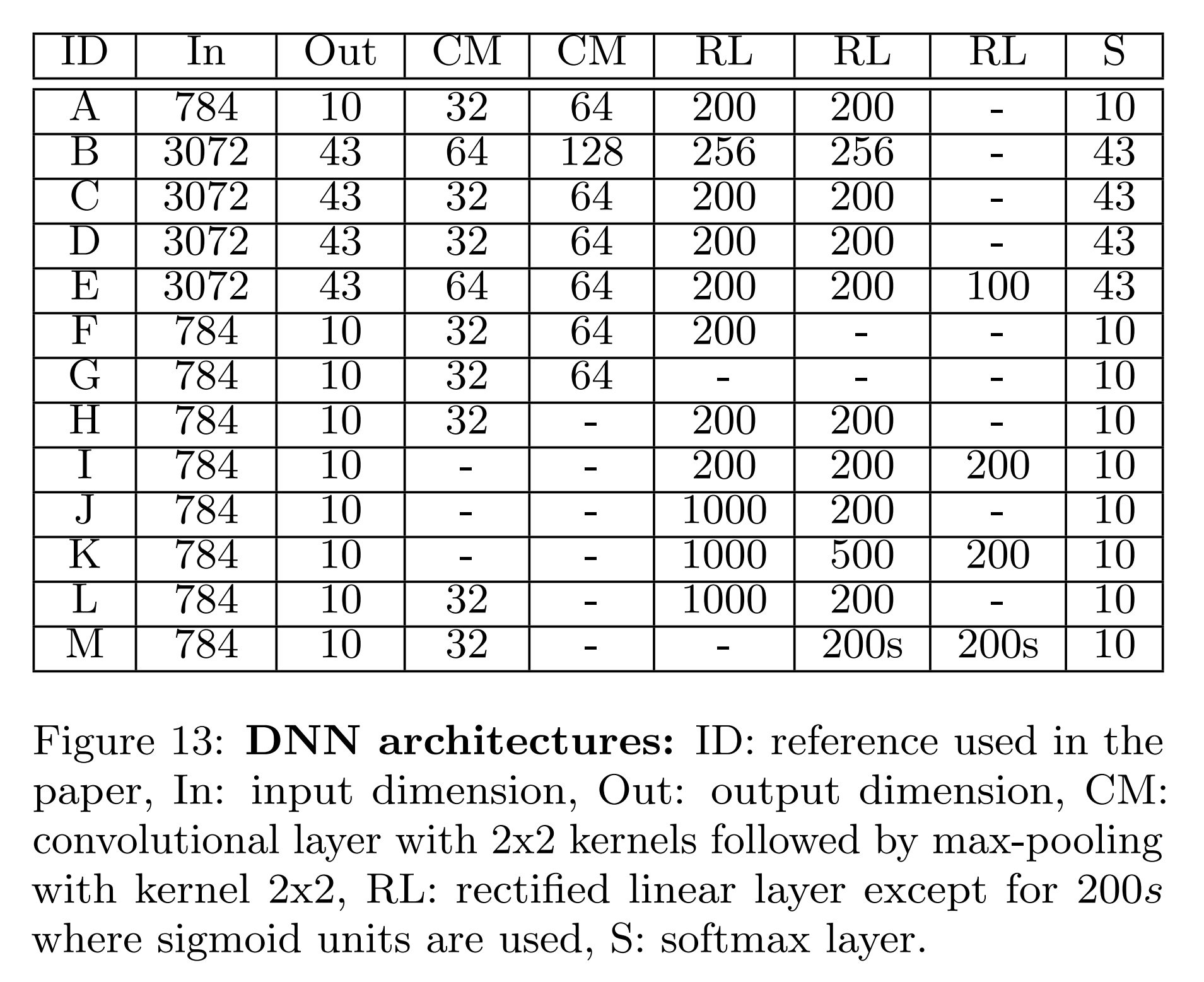
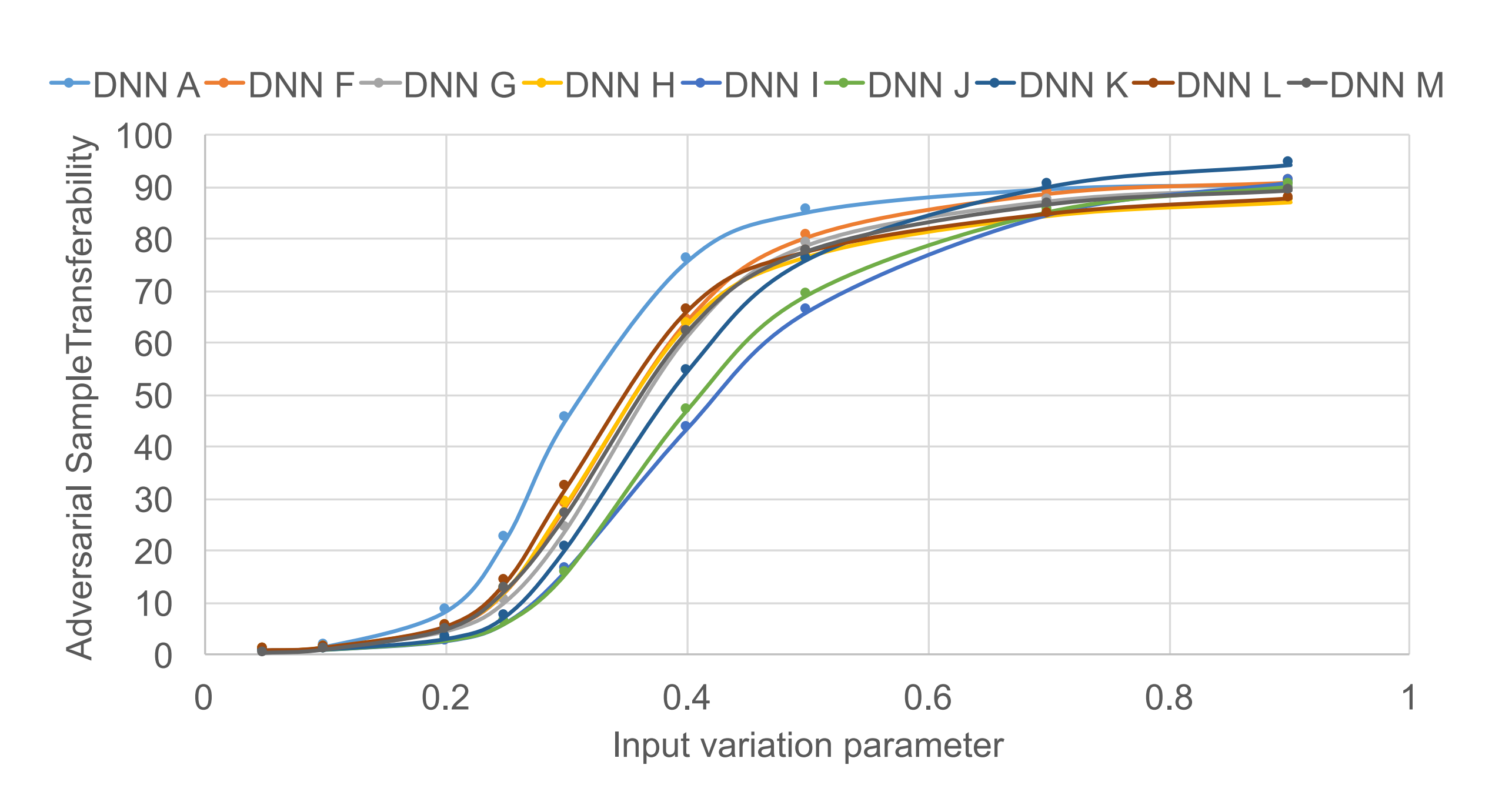
- FGSM FGSM modifies input data in a single step, with epsilon as the only adjustable parameter. According to the experimental results below, the pattern of increasing transferability with increasing epsilon was similar even when the model architecture changed. However, increasing epsilon makes changes human-perceptible, which limits this approach.
- Papernot Algorithm The maximum distortion \(\Upsilon\) is the proportion of input data components to modify, determined based on saliency values. And epsilon is the magnitude of modification to add to each selected component. These two parameters can be adjusted to improve the Papernot algorithm’s performance.
Adversarial Example Generation Comparison
FGSM and the Papernot algorithm differ in their adversarial example generation approaches. FGSM modifies all input components slightly at once, while the Papernot algorithm modifies only some input components significantly. This experiment examines the transferability difference between the two approaches at the same total perturbation. To this end, the L1-norm of total perturbation is fixed as follows:
\[\|\delta \mathbf{x}\|_{1}=\varepsilon\,\|\delta \mathbf{x}\|_{0}\]| FGSM | Papernot | |
|---|---|---|
| \(|\delta \mathbf{x} |_1\) | Total perturbation | Total perturbation |
| \(\varepsilon\) | \(\varepsilon\) | \(\varepsilon\) |
| \(|\delta \mathbf{x} |_0\) | \(1\) | \(\Upsilon\) |
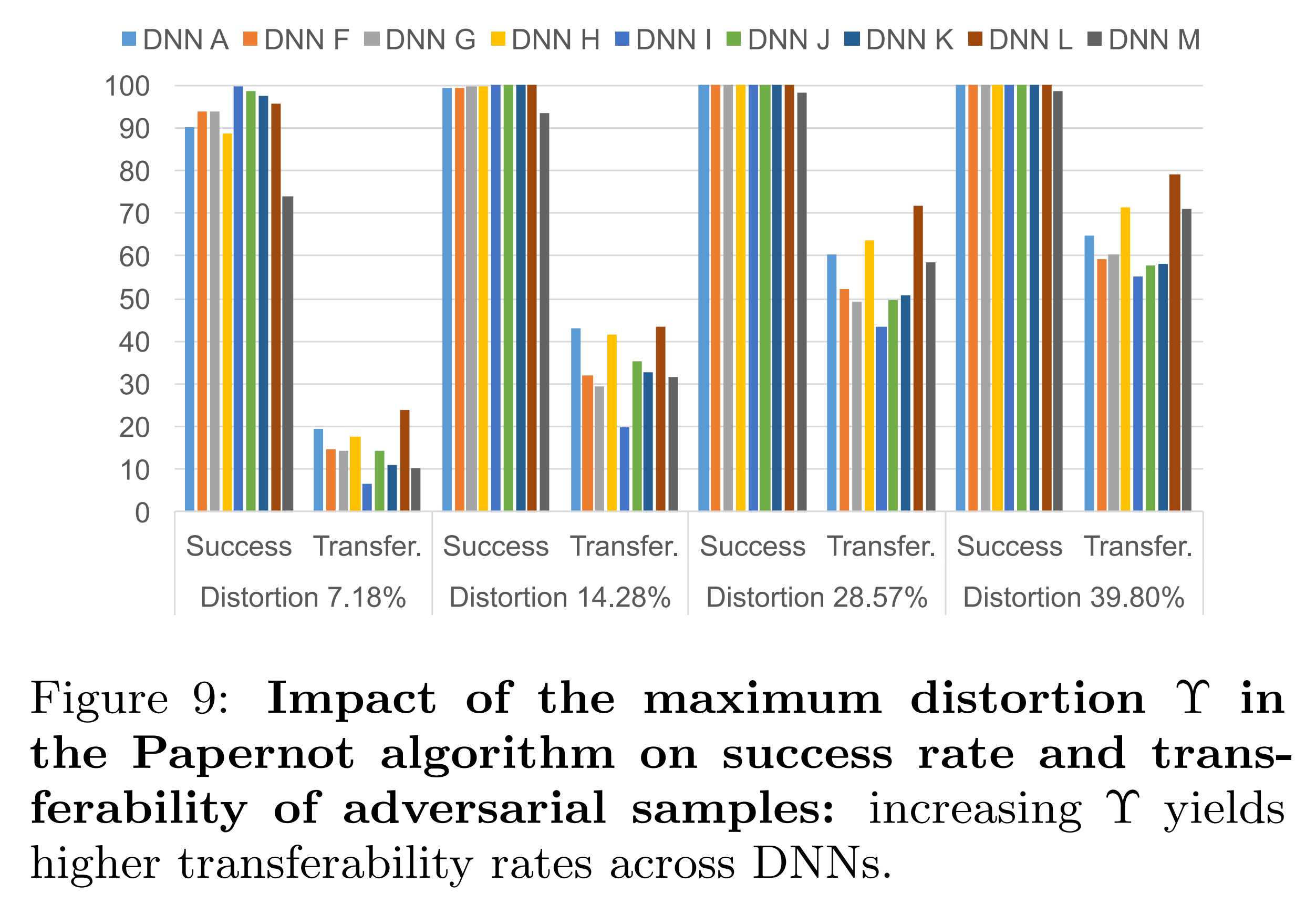
The above experimental results show the results when epsilon is fixed at 1 and only \(\Upsilon\) is adjusted. The substitute model’s transferability increases as \(\Upsilon\) increases.
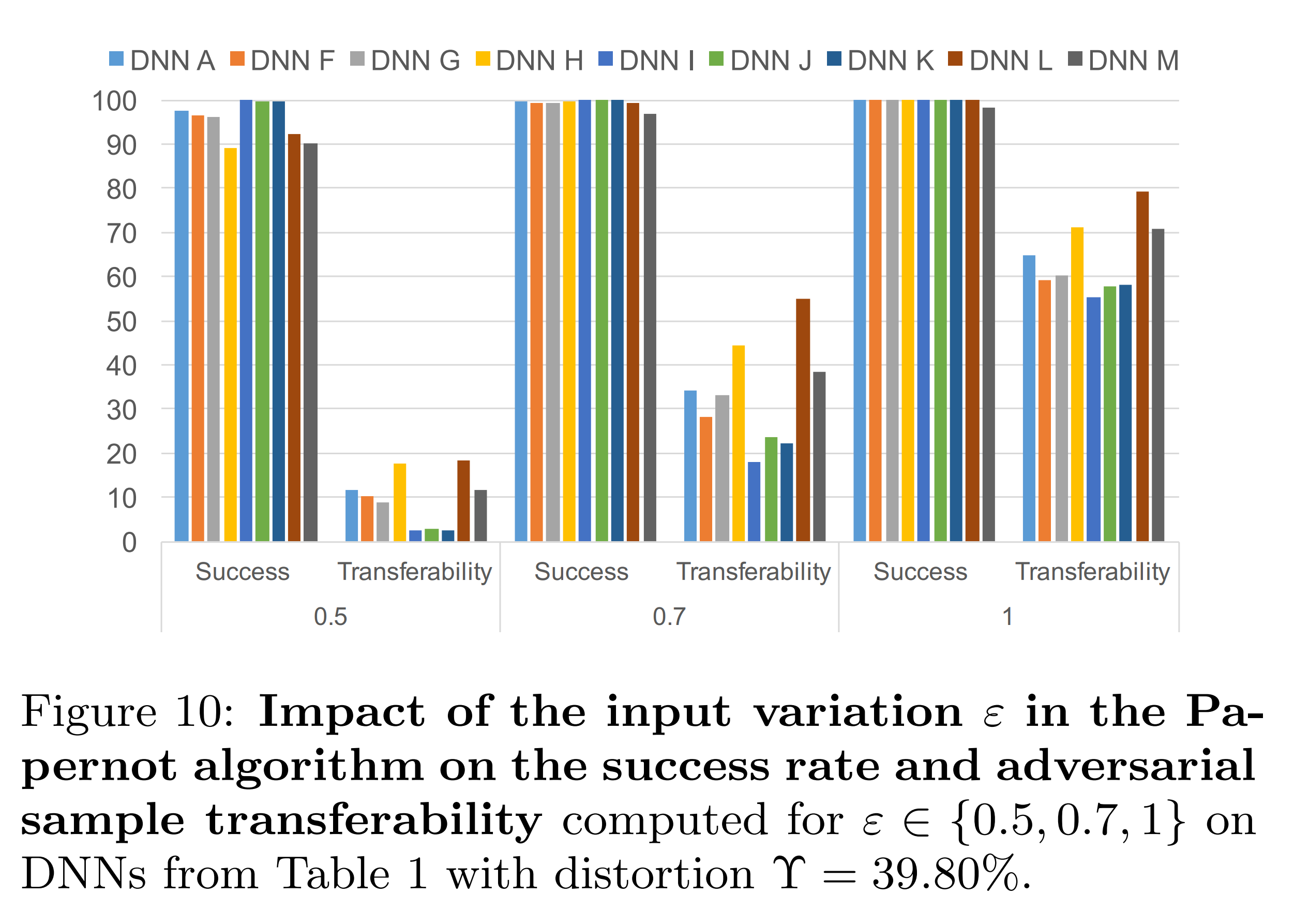
The above experimental results show the results when \(\Upsilon\) is fixed at 39.80% and only epsilon is adjusted. The substitute model’s transferability decreases as epsilon decreases. This is because, with \(\Upsilon\) fixed, the reduced modification magnitude could not be compensated.
Therefore, the paper concludes that the choice of adversarial example generation algorithm depends on the desired perturbation approach:
- FGSM: Slightly modifies all input components. Specializes in epsilon adjustment.
- Papernot Algorithm: Significantly modifies only some input components. Specializes in \(\Upsilon\) adjustment.
Generalization Experiments
Experimental Setup
All substitute models and oracles experimented with so far were DNN models. However, this experiment evaluates generalizability by testing in diverse settings. Accordingly, this experiment uses DNN and LR as substitute models, and DNN, LR, SVM, DT, kNN, and cloud remote models as oracles.
The initial training data for the substitute model is the MNIST test set, and PSS and RS techniques are also applied.
Substitute Model Training Generalization Performance
If the substitute model is differentiable, training is possible even if the oracle is non-differentiable like DT. The substitute model must be differentiable because synthetic samples need to be generated based on the Jacobian.
LR outputs a softmax probability vector, so the Jacobian can be computed in the same way as DNN, and it can be used as a substitute model.
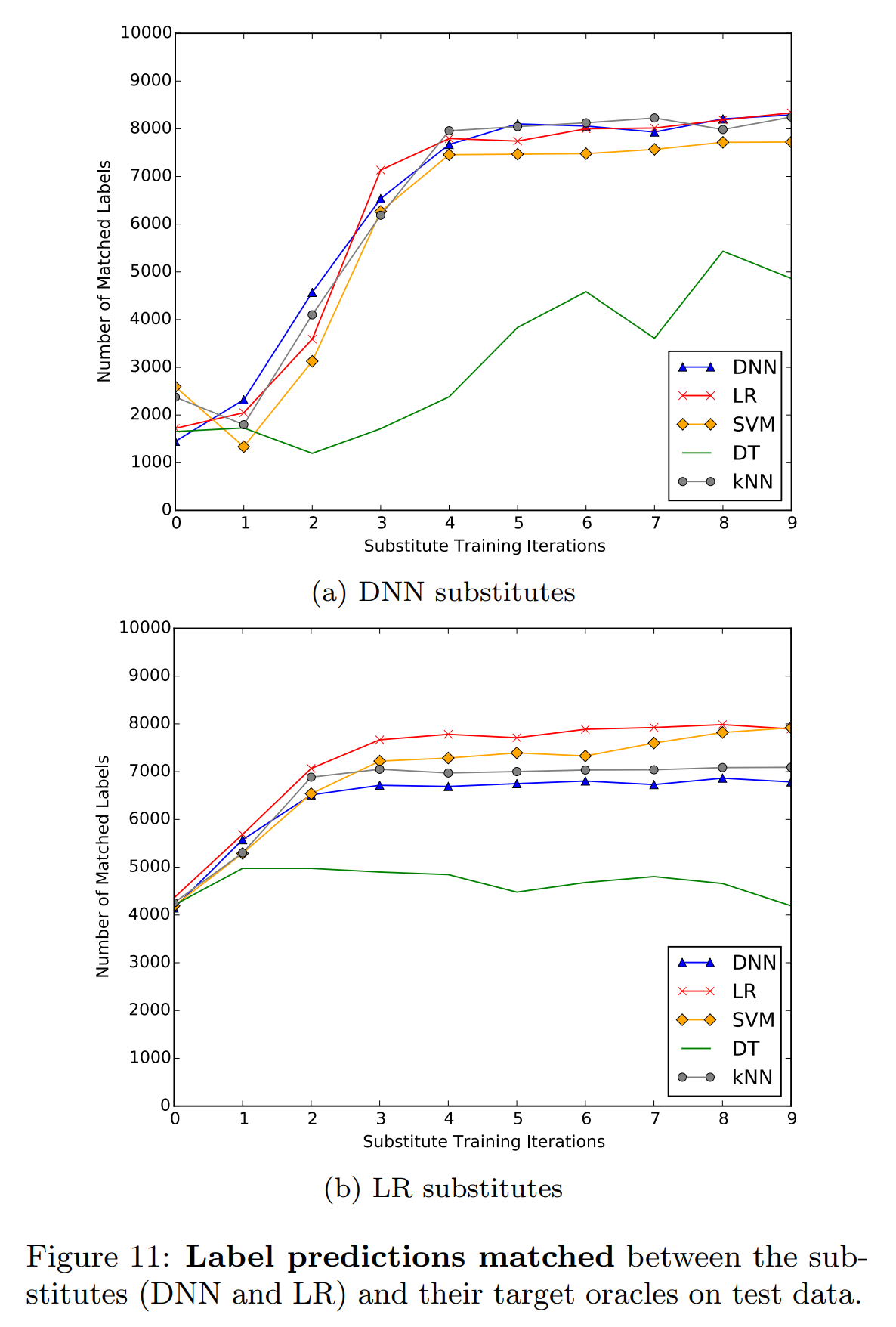
Looking at the two experimental results above, the LR substitute model’s performance is generally lower than the DNN substitute model. However, when the oracle is LR or SVM, the LR substitute model is superior. In particular, the LR substitute model tends to converge at earlier rounds.
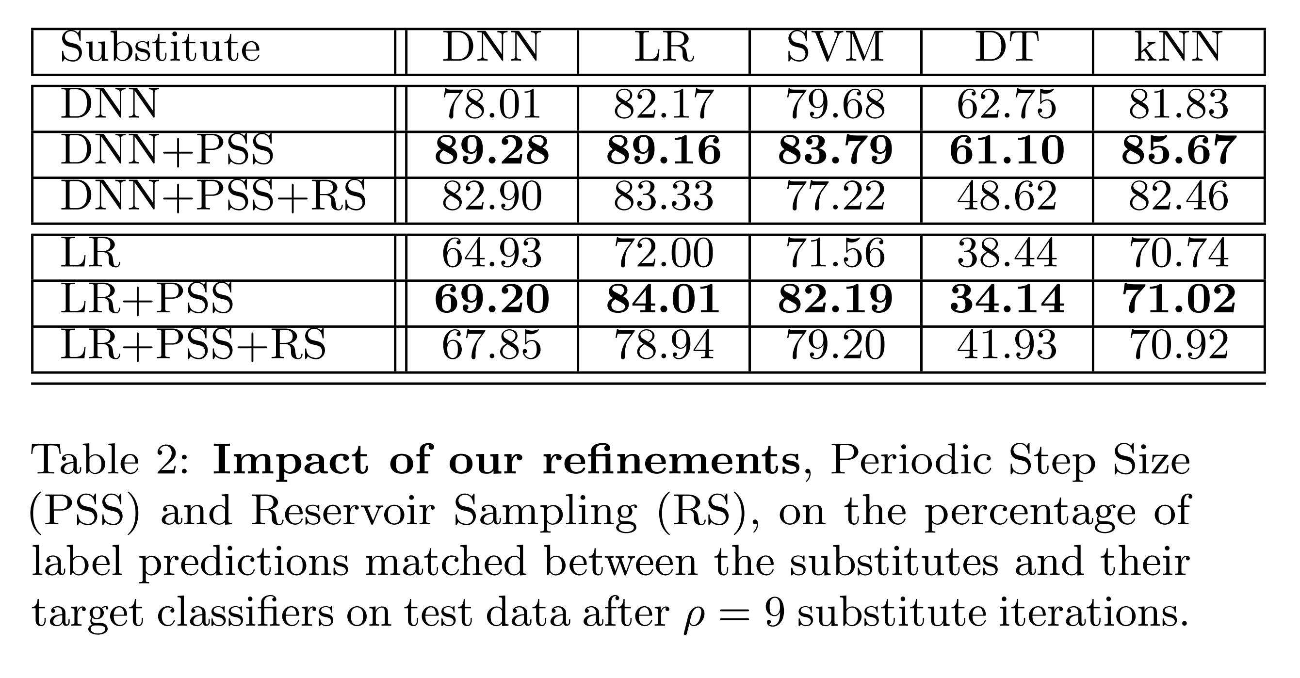
The results above show that prediction agreement between the substitute model and oracle improves significantly when using PSS. And when RS is used together with PSS, it shows superior performance compared to the vanilla approach.
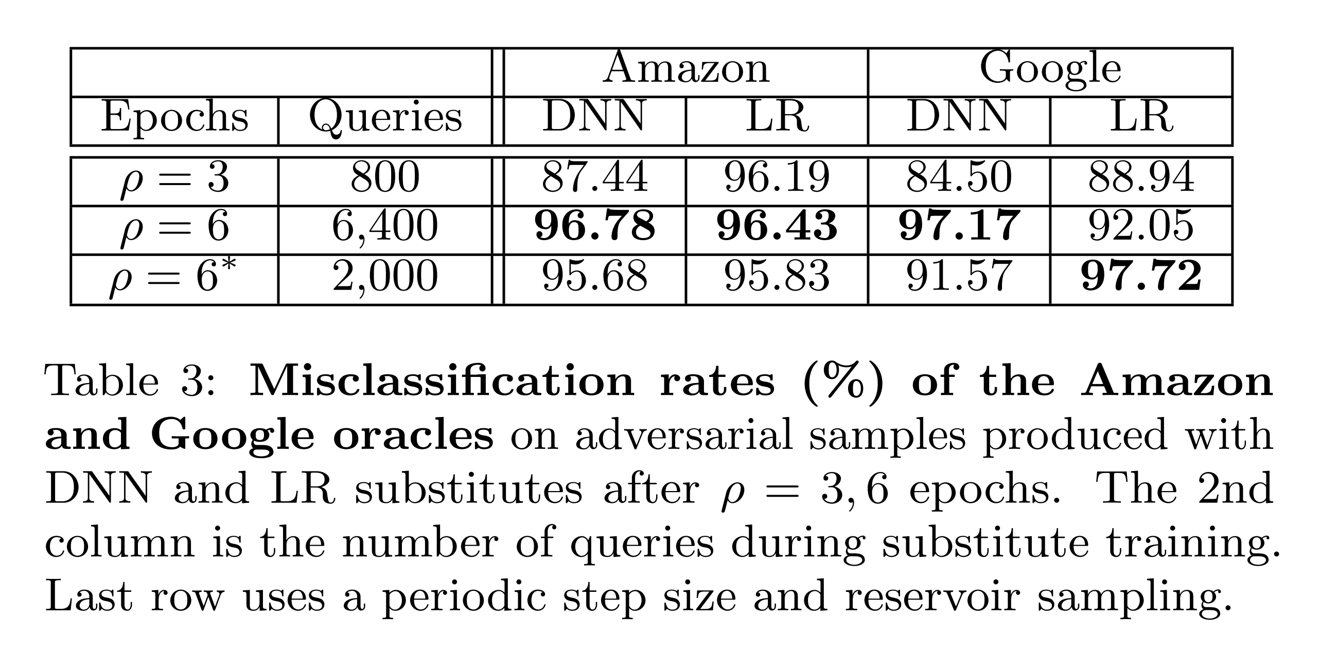
The above experiment shows the misclassification rate when generating adversarial examples using FGSM from the substitute model for 10,000 MNIST test set images and inputting them to the oracle.
Amazon and Google remote models are used as the oracle. The results show overall high misclassification rates. Furthermore, even though the number of oracle queries was reduced from 6,400 to 2,000 using PSS and RS, misclassification rates remained similar or even increased.
Defense Experiments
Background
Defenders use various defense strategies to protect model performance from these attacks. Adversarial example defense is divided into reactive approaches focused on attack detection, and proactive approaches that make the oracle itself more robust. Since this paper’s attack technique can distribute oracle queries across multiple attackers, it is difficult for the defender to detect the attack. Therefore, this defense experiment introduces defense techniques that make the oracle more robust and examines the attack performance of the proposed technique against them.
Gradient Masking
Many defense techniques fall under the category of gradient masking. Gradient masking modifies the oracle so that the attacker cannot obtain useful gradients from the oracle. This makes it difficult for the attacker to generate adversarial examples directly against the oracle.
However, even without knowing the oracle’s gradients, the attacker can bypass gradient masking by generating adversarial examples from a smoothed version of the oracle or from a substitute model. No defense technique is perfect, and this paper analyzes adversarial training and defensive distillation, which have been empirically proven effective.
Adversarial Training
Adversarial training is a technique that improves model robustness by inserting adversarial examples throughout the training process. This experiment trains the oracle adversarially on MNIST data and checks the attack success rate. For this purpose, adversarial examples were generated using FGSM at each batch, immediately included in the training data, and then the next batch was trained.
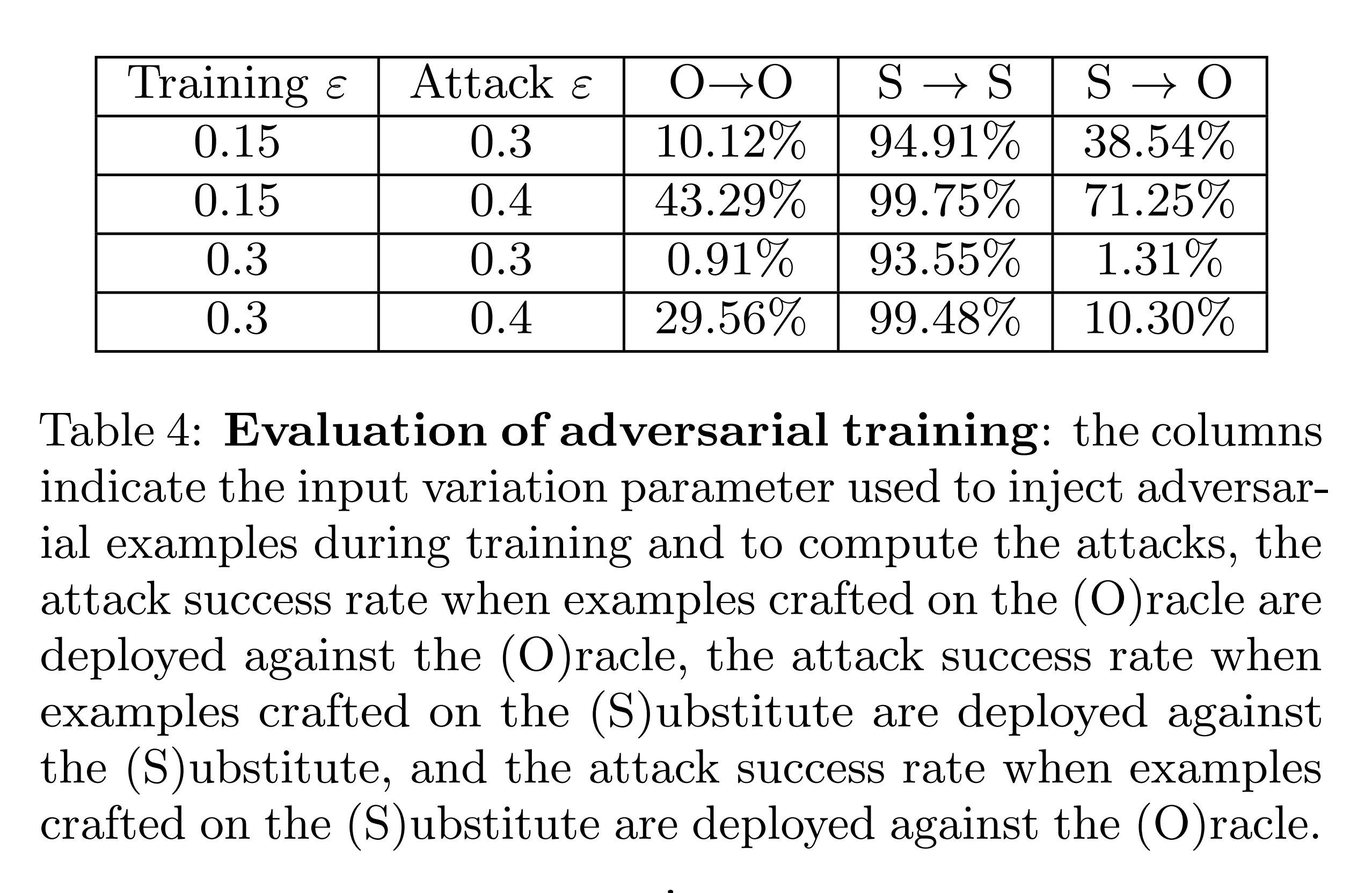
The experimental results above show that at \(\varepsilon=0.15\), adversarial examples generated from the substitute model fool the oracle up to 71.25%. This shows that adversarial training against small perturbations (\(\varepsilon=0.15\)) acts as a form of gradient masking and is vulnerable to substitute-model-based black-box attacks.
On the other hand, if the defender adversarially trains with larger perturbations like \(\varepsilon=0.3\), the model shows robustness against such black-box attacks.
Defensive Distillation
Defensive distillation is a gradient masking technique that distills the oracle to avoid leaking useful gradients to the attacker. This experiment distills an oracle trained on MNIST data and compares white-box and black-box attack success rates.
White-box attack: Generates adversarial examples using FGSM directly from the distilled oracle and inputs them to the distilled oracle.
Black-box attack: Generates adversarial examples using FGSM from a substitute model built from the distilled oracle and inputs them to the distilled oracle.
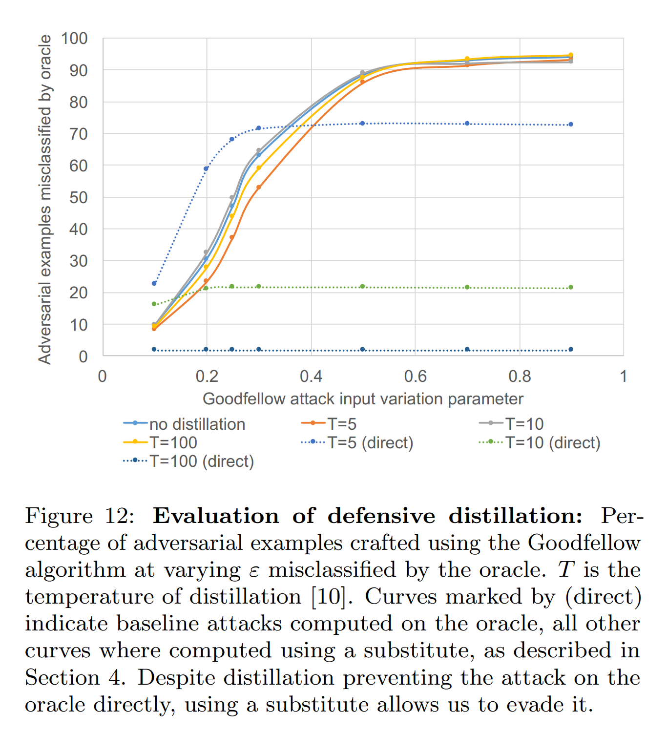
The graph above shows that defensive distillation provides effective defense against white-box attacks (direct). This is because the distillation process reduces the oracle’s gradients around training data, lowering FGSM’s effectiveness against the distilled oracle.
Conversely, against black-box attacks, defense performance is low regardless of the oracle’s distillation temperature \(T\). This is because the substitute model only takes labels, not gradients, from the distilled oracle, so the substitute model’s gradients are not reduced. As a result, the substitute model maintains sufficient gradients for FGSM attacks, leading to high black-box attack performance.
| Gradient Masking | Adversarial Training | Defensive Distillation | |
|---|---|---|---|
| White-box attack | Somewhat robust | Robust | Robust |
| Black-box attack | Vulnerable | Robust only with large perturbation training | Vulnerable |
Conclusion
This study is based on a black-box setting where the attacker can only query labels from the oracle without any information about the model’s internal structure or training data. Based on this, it proposed an attack technique that trains a substitute model using synthetic samples to deceive the oracle.
The attacker iteratively performs Jacobian-based augmentation using labels obtained through oracle queries, approximating the substitute model’s decision boundary close to the oracle’s. Adversarial examples generated from the substitute model were then transferred to the oracle. As a result, misclassification rates of 84.24% on remote DNNs, and 96.19% and 88.94% on Amazon and Google oracles were achieved, respectively. Moreover, it demonstrated excellent performance in neutralizing gradient masking-based defenses.
These achievements can contribute to enhancing the practicality of black-box attacks.