Paper: TOWARDS REVERSE-ENGINEERING BLACK-BOX NEURAL NETWORKS
Authors: Seong Joon Oh, M. Augustin, M. Fritz, and B. Schiele
Venue: International Conference on Learning Representations (ICLR), Vancouver, B.C., Canada, 2018
Introduction
A black-box model is a model where only the output for a given input can be observed, and internal attributes such as the internal workings or structure are unknown. Conversely, a white-box model is one where all internal attributes are known.
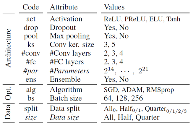
Here, model attributes refer to the model’s architecture, including the model type, network depth and connectivity, activation functions, etc., the optimization process used during training, and characteristics and distribution information of the training data.
Many models are designed and deployed as black-box models to protect intellectual property and the privacy of training data.
However, black-box models whose internal attributes are not disclosed can have their internal attributes inferred through reverse engineering techniques.
Inferred internal attributes can be used to generate more sophisticated adversarial samples, posing a threat to the model.
Conversely, they can also be utilized to generate adversarial samples for privacy protection purposes against content with privacy concerns, such as facial images.
This paper proposes how reverse engineering can be performed on black-box models, analyzes it through experiments, and verifies whether the proposed method has generalization potential across various models and situations through additional experiments.
Main Content
Experimental Objective
The experiments in this paper aim to infer the internal attributes of a black-box model using the output values obtained from input queries.
Meta Training Set & Metamodel
To infer a specific black-box model, a dataset is first constructed by collecting various white-box models that are expected to be similar to the black-box model to a certain degree. This is called the meta-training set.
Subsequently, another model is trained that takes the output values of various white-box models as input and outputs the attributes of those models. This is called the metamodel.
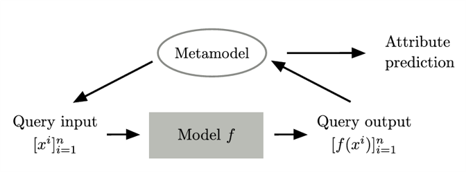
The final metamodel structure proposed in this paper is shown in the figure. For the black-box model to be predicted, the metamodel generates n ideal input queries, and the output values from passing these input queries through the black-box model are fed back into the metamodel as input, ultimately producing predictions about the model’s attributes.
The metamodel comes in three variants: KENNEN-O, KENNEN-I, and KENNEN-IO.
KENNEN-O
KENNEN-O predicts all model attributes at once from N fixed input queries. The input queries are randomly sampled from the dataset and remain unchanged, being used in both the training and evaluation phases. The overall training structure is shown in the following figure.
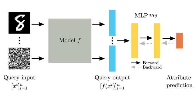
N fixed queries are input to the meta-training models (white-box models), and their output values are concatenated in an order-sensitive manner and fed into classifier m, which is trained to predict the attributes of the black-box model.
This training process is expressed by the following formula.
\[\min_{\theta} \ \mathbb{E}_{f \sim \mathbb{F}} \left[ \sum_{a=1}^{12} \mathcal{L} \left( m_\theta^a \left( \left[ f(x^i) \right]_{i=1}^{n} \right), y^a \right) \right]\]With 12 attributes, the Cross Entropy Loss between the predicted and actual labels for all attributes is summed for each meta-training data sample, and the parameters are optimized to minimize the expected value over the entire model distribution.
The classifier consists of an MLP (multilayer perceptron) with two hidden layers of 1000 hidden units each, and the output layer consists of 12 parallel linear classifiers (12-Linear Classifiers) for each attribute.
The classifier’s output is expressed by applying argmax to the softmax values for each attribute.
Let me explain with an example.
Assume there are 3 attributes to predict:
- Attribute A: 3 classes
- Attribute B: 2 classes
- Attribute C: 4 classes
Each attribute is predicted as a probability distribution through softmax.
| Attribute | Classes | Softmax Output |
|---|---|---|
| A | 3 | [0.1, 0.7, 0.2] |
| B | 2 | [0.6, 0.4] |
| C | 4 | [0.25, 0.1, 0.5, 0.15] |
Each softmax value is then converted to a single integer value through argmax, and the prediction for each attribute is output as the final prediction result.
# Compute argmax for each attribute's softmax output
[
  argmax([0.1, 0.7, 0.2])      # → 1
  argmax([0.6, 0.4])           # → 0
  argmax([0.25, 0.1, 0.5, 0.15]) # → 2
]

# Final prediction result
[1, 0, 2]
KENNEN-O is applicable not only to neural network-based models but also to non-neural network-based models.
KENNEN-I
Unlike KENNEN-O, KENNEN-I takes only one input query at a time and learns to predict model attributes one at a time individually. While KENNEN-O optimizes the parameters of classifier m, KENNEN-I is trained by optimizing individual input queries.
The KENNEN-I model structure is shown in the following figure.
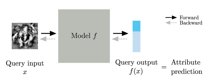
Unlike KENNEN-O, which trains a separate classifier m by passing the output values of meta-training models through an MLP structure to predict all attributes, KENNEN-I optimizes input queries such that when a single input query is fed into a meta-training model, the model’s output value itself represents the prediction for the specified attribute. The learning objective of KENNEN-I can be expressed as follows.
\[\min_{x\colon \text{image}} \ \mathbb{E}_{f \sim \mathbb{F}} \left[ \mathcal{L} \left( f(x), y^a \right) \right]\]Let me explain the operation of KENNEN-I with an example. Assume the black-box model to be predicted is an MNIST Digit Classifier, the attribute to predict with KENNEN-I is the number of convolutional layers, and the possible values are 2, 3, or 4 layers. The number of convolutional layers (2, 3, 4) is represented by labels (0, 1, 2) respectively.
For a typical digit image input, the MNIST digit classifier outputs softmax values representing probabilities for 10 digits, where each softmax value indicates the probability that the image is of that digit, and finally outputs the digit with the highest probability through argmax.
| Model | f(x) | Argmax | Meaning |
|---|---|---|---|
| f | [0.89, 0.02, 0.02, …, 0.03] | 1 | Predicted digit = 1 |
However, when an input query optimized through KENNEN-I enters black-box model g, the output is still expressed as softmax values for 10 digits, but each softmax value now represents the probability for the corresponding attribute set during training.
In this example, since the number of convolutional layers (2, 3, 4) was mapped to labels (0, 1, 2), if the argmax of g(x)’s softmax yields 0, the meaning is not that the input image is predicted to be the digit 0, but rather that the black-box model has 2 convolutional layers.
| Model | Attribute | Ground Truth label | g(x) | Argmax | Meaning |
|---|---|---|---|---|---|
| g_1 | #Conv layer : 3 | 1 | [0.01, 0.89, 0.02, …, 0.03] | 1 | Model has 3 Conv layer |
| g_2 | #Conv layer : 2 | 0 | [0.87, 0.04, 0.02, …, 0.01] | 0 | Model has 2 Conv layer |
KENNEN-I is useful in that it enables attribute inference from simple input-output pairs, but it also has several limitations.
First, since the model must be trained individually for each attribute, it is difficult to predict all attributes at once.
Second, prediction is impossible when the attribute has more classes than the model’s output dimension.
Third, the optimized input values through the model may differ from normal inputs, making it vulnerable in terms of stealth (detection evasion).
To address these limitations, the KENNEN-IO model is proposed, which combines KENNEN-I and KENNEN-O.
KENNEN-IO
KENNEN-IO includes both the process of optimizing n input queries and the process of optimizing classifier m.
The learning objective of KENNEN-IO can be expressed as follows.
\[\min_{\{x^i\}_{i=1}^{n} \, \text{: images}} \ \min_{\theta} \ \mathbb{E}_{f \sim \mathbb{F}} \left[ \sum_{a=1}^{12} \mathcal{L} \left( m_\theta^a \left( \left[ f(x^i) \right]_{i=1}^{n} \right),\ y^a \right) \right]\]The above formula means that n input queries and meta-classifier m are simultaneously trained to minimize the average Cross Entropy.
The training approach first trains classifier m using the KENNEN-O method for the initial 200 epochs.
Then, for an additional 200 epochs, the n input queries and the classifier’s parameters are alternately updated every 50 epochs.
KENNEN-IO is an advanced metamodel structure that integrates the query optimization of KENNEN-I with the simultaneous prediction of all attributes from KENNEN-O.
Experiment
Experimental Setup
To test and validate the above models, this paper uses MNIST Digit Classifiers as both the black-box models and meta-training models (white-box models). There are 12 attributes in total, with various values for each attribute used to construct diverse meta-training models.
The total number of possible combinations of the 12 attributes is 18,144. By setting the random seed from 0 to 999 (1000 values), a total of 18,144,000 MNIST sets were created. From these, 10,000 models were randomly selected and trained on MNIST. Models with accuracy below 98% were removed, and ensembles were constructed based on identical architectures, resulting in a final set of 11,252 models.
The extracted models were divided into 5,000 for training, 1,000 for evaluation, and the remaining 5,252 models.
Two methods were used to split the models.
The first method is Random Split. This method simply divides the models randomly.
The second method is Extrapolation Split. This method intentionally creates a domain gap between training and evaluation data to assess whether the metamodel works well even on black-box models different from those used in training.
Example:
Using
#layers(number of convolutional layers) as the criterion,Shallow models (e.g.,
#layers < 10) → Meta-training setDeep models (e.g.,
#layers ≥ 10) → Test set
By splitting based on attributes in this way, it is possible to measure generalization performance – whether the model can make predictions about structures it has never seen during training.
Training and Evaluation
Let us first examine the evaluation metrics after training and evaluation using the Random (R) Split method.
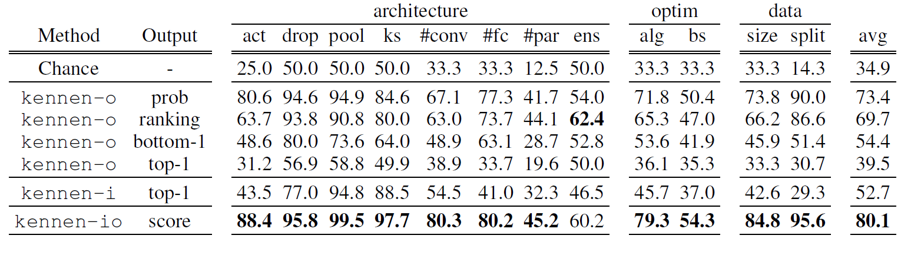
The Output column in the table above refers to the values used from the meta-training models’ outputs, with each meaning as follows:
prob: Uses the full softmax probability vector as input ranking: Uses the descending order of classes by softmax probability bottom-1: Uses only the class with the lowest probability top-1: Uses only the class with the highest probability score: A summary statistic based on the softmax probability vector
Examining the evaluation results, all models show better performance than Random Guess.
Furthermore, KENNEN-O using bottom-1 output has a higher average prediction rate than KENNEN-O using top-1 output.
Finally, the KENNEN-IO model shows better predictions for nearly all attributes compared to other models.
Next, let us examine the evaluation metrics after training and evaluation using the Extrapolation (E) Split method.
When using this split method, performance must be evaluated with metrics other than standard accuracy. This is because some attribute classes may not exist in the training data at all, appearing only in the evaluation data. Therefore, the attribute used as the split criterion is excluded from evaluation, and prediction accuracy is measured only for the remaining attributes.
Example:
Full attribute set A = {A1, A2, A3, A4}
Split criterion attribute A’ = {A1}
Attributes used for E split accuracy measurement: A \ A’ = {A2, A3, A4}
After measuring E-Split Accuracy, Normalized Accuracy is computed to evaluate how well this method performs compared to Random Split. The formula and evaluation results are as follows.
\[\text{N.Acc}(\tilde{A}) = \frac{\text{E.Acc}(\tilde{A}) - \text{Chance}(\tilde{A})} {\text{R.Acc}(\tilde{A}) - \text{Chance}(\tilde{A})} \times 100\%\]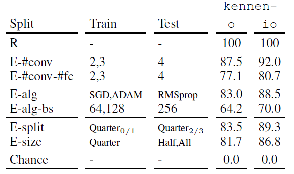
The above metrics show the normalized accuracy for each attribute and model used in the E-Split. While all N.Acc values are below 100%, indicating E-Split Accuracy is lower than R-Split, all show performance above 70%, demonstrating that the E-split method is effective even when there is a domain gap between the black-box model and the meta-training models.
Additionally, KENNEN-IO showed approximately 5% better performance than KENNEN-O in all experimental cases.
Additional Analysis
In addition to normalized accuracy, Confusion Matrices were analyzed to revalidate whether the accuracy results are meaningful.
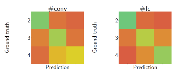
The diagonal elements where actual and predicted values match appear in deeper green, indicating better predictions, while off-diagonal elements appear in lighter to deeper red. Examining the figure, models with adjacent numbers of convolutional layers (i.e., 2 and 3, or 3 and 4) show lighter red confusion compared to models with 2 and 4 layers. This means that adjacent numbers of convolutional layers are more easily confused.
This has two implications.
First, semantic attribute information (number of layers, number of parameters, batch size, etc.) actually exists within the neural network output.
Second, the metamodel can generalize by learning semantic information rather than simply relying on artifacts.
Thus, by analyzing both normalized accuracy and confusion matrices, it was demonstrated that the experiments yield meaningful results.
Additional Experiments
In addition to the MNIST digit classifiers used in the experiments, additional experiments were conducted with ImageNet classifiers to demonstrate that the metamodel can also be applied to realistic image classification.
In this experiment, KENNEN-O was used as the metamodel, and the models used for training/evaluation consisted of 5 different model families, including different versions within each family, for a total of 19 models.
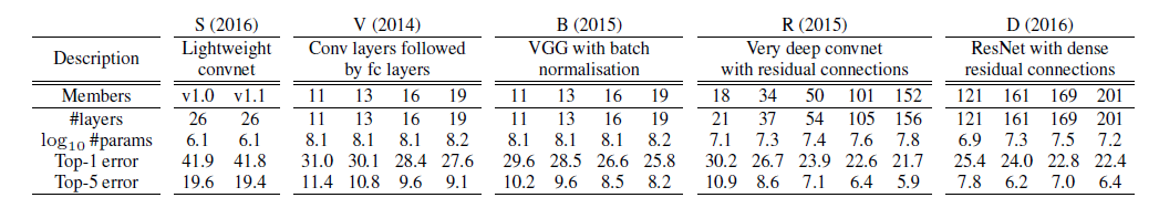
The attribute evaluated was the model family, with a total of 5 classes (S, V, B, D, R).
After training the metamodel KENNEN-O based on the above models, accuracy was evaluated by averaging the results of each model on how well the model family was predicted.
To reliably validate the model’s performance, evaluation was conducted as follows.
-
Cross Validation
- In each experiment, one test network was randomly sampled from each model family.
- This was repeated 10 times to obtain stable evaluation results.
-
Random query sampling from ImageNet validation set
- Queries were randomly sampled from the ImageNet validation dataset.
- 10 random query sets were selected for each experiment.
Evaluation with a total of 100 query sets yielded an average accuracy of 90.4%.
When the number of query sets was increased to 1000, the average accuracy rose to 94.8%.
Subsequently, additional experiments were conducted to verify how much the model attribute prediction through the metamodel can make models more vulnerable to Adversarial Image Perturbations (AIPs).
In adversarial image perturbation attacks, transferability refers to the ability of adversarial examples generated from one model to successfully cause misclassification in other models.
In this additional experiment, the concept of transferability was applied to verify the assumption that if the metamodel can predict a model’s family, the model becomes more vulnerable.
Experimental results showed that adversarial examples generated within the same model family (within-family) had higher attack success rates (misclassification rates), while cross-family transferability was relatively less effective.
Additionally, the study examined how misclassification rates differ across scenarios when adversarial image perturbation attacks are conducted.
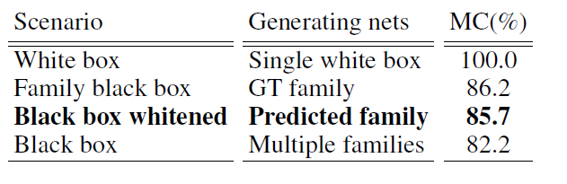
The experimental results show that white-box models had a 100% misclassification rate, and the misclassification rate of black-box models whose family was predicted through the metamodel was similar to that of black-box models whose family was already known.
This suggests that the metamodel can accurately predict the model’s family, that this can provide an important clue to attackers, and that attackers can leverage this information to design more sophisticated and effective adversarial attacks.
Conclusion
The metamodel proposed through this research demonstrated that it can effectively predict various attributes of black-box models using only input-output query sets. The proposed model inferred structural features of the model, such as the number of convolutional layers, the number of fully connected layers, the optimization method, and the data size, without any internal information.
Furthermore, it was demonstrated through transferability experiments that reverse-engineering the attributes of a black-box model can make it more easily exposed to adversarial attacks, as evidenced by the significantly higher attack success rates observed for models within the same family.
These results mean that the fact that metamodels can predict model attributes can provide important clues to attackers. Ultimately, attackers can use this information to design more sophisticated and effective adversarial samples.
Therefore, when designing and deploying black-box models, additional defensive measures against attribute inference attacks are needed from a security perspective, beyond just performance considerations.