Paper: Unified Gradient-Based Machine Unlearning with Remain Geometry Enhancement
Authors: Zhehao Huang, Xinwen Cheng, JingHao Zheng, Haoran Wang, Zhengbao He, Tao Li, Xiaolin Huang
Venue: 38th Conference on Neural Information Processing Systems (NeurIPS 2024)
URL: https://openreview.net/forum?id=dheDf5EpBT&referrer=%5Bthe%20profile%20of%20Tao%20Li%5D
Background
Research Trends in Machine Unlearning
“Machine Unlearning” aims to remove the influence of specific data from a pre-trained model. It is commonly used when knowledge is no longer up-to-date, when biases exist, and to prevent text-to-image models from generating not-safe-for-work (NSFW) images.
Existing machine unlearning methods are divided into two approaches: Exact MU and Approximate MU. Exact MU can be achieved by retraining (RT) from scratch on a dataset without the forget data. However, this method is not time-efficient and requires significant computational resources when applied to large-scale models. Therefore, recent research aims to achieve performance as close as possible to a retrained model using Approximate MU.
Limitations of Euclidean Distance-based Measurement
Existing Approximate MU finds the steepest descent gradient under the concept of Euclidean distance during gradient descent. However, this method has the problem of not considering the relative importance among parameters.
Recent research results show that model parameters and the training process are primarily embedded in a low-dimensional manifold. This reveals a problem with the Euclidean distance measurement approach, where changes between parameters occurring on a specific manifold are not reflected in the output space.
This paper resolves this problem by computing the descent direction using a KL divergence distribution based on the second-order Hessian matrix of the remaining data. However, computing the Hessian itself can also be resource-intensive for large-scale models. Therefore, the paper proposes a fast-slow weight method that approximates the Hessian approach but dynamically allocates parameters rather than fixing the initially computed parameters.
Approximate MU from the Perspective of Steepest Descent
Euclidean Distance-based Approximate MU
Steepest descent computes the direction in which a function F decreases most rapidly within a certain range. This can be expressed as the following equation.
\[\begin{equation} \delta \theta := \arg\min_{\substack{\ \rho(\theta_t, \theta_t + \delta\theta) \leq \xi}} F(\theta_t + \delta\theta) \end{equation}\]This can be expressed as the following equation.
\[\begin{equation} \theta_{t+1} = \arg\min_{\theta_{t+1}} \left[ F(\theta_{t+1}) + \frac{1}{\alpha_t(\xi, \theta_t)} \rho(\theta_t, \theta_{t+1}) \right] \end{equation}\]The distance function is also defined based on Euclidean distance as follows.
\[\rho(\theta_t, \theta_{t+1}) = \frac{1}{2} \|\theta_t - \theta_{t+1}\|^2\]KL Divergence-based Approximate MU
A loss function in the form of minimizing the difference between two probability distributions according to KL divergence rather than using a distance function can be defined as follows.
\[\begin{equation} \theta_{t+1} = \arg\min_{\theta_{t+1}} \left[ D_{KL} \big( p_z(\theta_*) \| p_z(\theta_{t+1}) \big) + \frac{1}{\alpha_t} \rho(\theta_t, \theta_{t+1}) \right] \end{equation}\]The above equation can be divided into three parts according to their functions.
\[\begin{equation} \theta_{t+1} = \arg\min_{\theta_{t+1}} \underbrace{D_{KL} \big( p_z^f(\theta_*) \| p_z^f(\theta_{t+1}) \big)}_{(a)} + \underbrace{D_{KL} \big( p_z^r(\theta_*) \| p_z^r(\theta_{t+1}) \big)}_{(b)} + \underbrace{\frac{1}{\alpha_t} \rho(\theta_t, \theta_{t+1})}_{(c)} \end{equation}\]The role of each part is as follows.
(a): The part that removes the influence of forget data
(b): The part that maintains the performance on remaining data
(c): The part that controls the size of each update
The researchers define the distance function using Newton’s direction reflecting the Hessian, rather than the Euclidean-based approach, to balance the influence of forget data and remaining data.
\[\begin{equation} \theta_{t+1} - \theta_t \approx -\alpha_t \underbrace{ \left[ H_f^* (H_r^*)^{-1} \right]}_{(S)}\underbrace{ \left[ -\nabla L_f(\theta_t; \epsilon_t) \right] }_{(F)} + \underbrace{\nabla L_r(\theta_t)}_{(R)} \end{equation}\](F) removes the influence of forget data by increasing its loss, and (R) controls the model to maintain its existing performance by minimizing the loss on remaining data.
(S) amplifies the updates on forget data while reducing updates on remaining data, adjusting the influence between the two datasets.
Existing machine unlearning methods missed one or more of the three elements (F), (R), and (S).
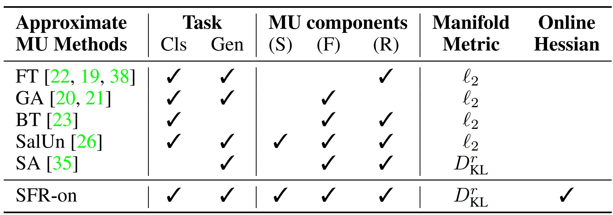
For example, Fine-Tuning did not consider the (F) element, making it difficult to guarantee effective unlearning performance. Gradient Ascent did not consider the (R) element, making it difficult to guarantee performance on the non-removed dataset. Random Labeling and BadTeacher Knowledge Distillation did not consider the (S) element, so while unlearning performance could be guaranteed, maintaining performance on remaining data was difficult.
Finally, the most recently published SalUn partially considered (S) by introducing the weight saliency concept, but lacked theoretical justification.
This paper emphasizes the difference from previous methods by presenting an unlearning method that considers all three elements.
Remain-Preserving Manifold
To effectively remove the data that needs to be removed while maintaining the model’s overall performance, the KL divergence-based Remain-Preserving Manifold concept is introduced.
This method resolves the issues with the existing Euclidean distance-based update size control approach and can adjust updates in a direction that does not significantly change the model output based on the variation between two probability distributions.
\[\begin{equation} \theta_{t+1} - \theta_t \approx -\tilde{\alpha}_t \underbrace{ (H_r^t)^{-1}}_{(R)} \underbrace{ \left[ H_f^* (H_r^*)^{-1} \right] }_{(S)} \underbrace{ \left[ -\nabla L_f(\theta_t; \epsilon_t) \right] }_{(F)} \end{equation}\]Elements of SFR-on
Hessian Approximation
When introducing the Remain-preserving manifold approach, the large computational cost of Hessian computation becomes a problem. Previous research has also attempted to approximate the Hessian using Fisher information, Fisher diagonal, and Kronecker-Laplace approximation, among others. The Selective Amnesia method used Fisher diagonal to approximate the Hessian, but since this approximation was fixed, errors accumulated during the unlearning process.
The paper solves the above problem using fast-slow weight updates.
Optimization Method Using Hessian Approximation (R-on)
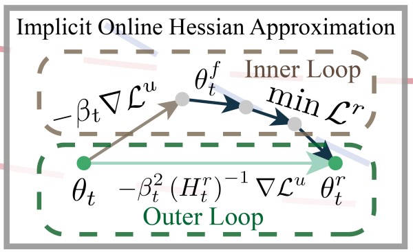
To address the problems of the method that adjusts the unlearning direction using the Hessian (implicit Hessian approximation), the paper proposes a fast-slow weight update method that obtains values approximating the Hessian without directly computing it.
The fast-slow weight update is divided into a fast weight update method that performs unlearning and a slow weight update method that minimizes the performance degradation caused by it. The model performs the slow weight update after the fast weight update to obtain parameters that guarantee unlearning performance while maintaining model performance on remaining data.
Fast Weight Update
The fast weight update computes the gradient of the loss function on forget data to quickly update parameters in the direction that causes the model to forget the data.
\[\begin{equation} \quad \theta^f_t = \theta_t - \beta_t \nabla L^u (\theta_t) \end{equation}\]Slow Weight Update
The slow weight update maintains performance on remaining data through Fine-Tuning after the fast weight update. It optimizes by minimizing the loss function value on remaining data using the parameters obtained from the fast weight update.
\[\begin{equation} \min_{\theta^f_t} L^r (\theta^f_t) \quad \ \end{equation}\]Fast-Slow Weight Update
The update considering both methods above is as follows. Instead of directly computing the Hessian, the fast-slow weight method is introduced to approximately apply the inverse of the Hessian.
\[\begin{equation} \theta_t - \theta^r_t \approx \beta_t^2 \left[ \nabla^2 L^r (\theta_t) \right]^{-1} \nabla L^u (\theta_t) = \beta_t^2 (H_t^r)^{-1} \nabla L^u (\theta_t). \end{equation}\]This approach weakens parameter updates in directions that would significantly damage performance on forget data, and strengthens updates in directions with less impact. In other words, by introducing the Hessian rather than simply summing loss function gradients, the model’s performance on remaining data can be maximally preserved.
Weight Adjustment Method (F)
In existing unlearning methods, all samples have equal importance, meaning they have equal contribution to the loss function during unlearning. However, depending on importance, some samples can be easily forgotten with a single update, while others may not be forgotten even after multiple updates.
The paper solves this problem by assigning different weights according to the importance of samples. The weights based on importance are defined as follows.
\[\begin{equation} \tilde{\epsilon}_{t,i} = \left( 1 - \frac{t}{T} \right) \frac{\frac{1}{\left[ \ell(\theta_t; z^f_i) \right]_{detach} ^\lambda}} {\sum\limits_{z^f_j \in D_f} \frac{1}{\left[ \ell(\theta_t; z^f_j) \right]_{detach}^\lambda}} \times N_f, \quad 1 \leq i \leq N_f \end{equation}\]The weights have the following properties.
- In the initial model, all data are assigned equal weights = 1.
- When unlearning is complete, all should have equal weights = 1.
- The larger the loss for specific data, the smaller the weight assigned.
Through the above process, updates are made by progressively reducing the loss.
Weight Saliency Method (S)
The paper introduces the weight saliency concept to balance the forget dataset and remaining data.
In the existing SalUn machine unlearning method, only parameters affecting forget data were considered. However, since this can damage performance on remaining data, a weight saliency method that considers both types of data is needed.
The weight saliency map is as follows.
\[\begin{equation} m = I \left[ \frac{F^f_{\text{diag}}}{F^r_{\text{diag}}} \geq \gamma \right], \quad \text{where} \quad F^f_{\text{diag}} = [\nabla L^f (\theta_0)]^2, \quad F^r_{\text{diag}} = [\nabla L^r (\theta_0)]^2. \end{equation}\]The weight saliency map is applied only to forget data so that updates occur only for important samples that need to be forgotten.
SFR-on
The paper presents SFR-on, which integrates the three elements S, F, and R-on into one.
The updates in SFR-on can be divided into the fast weight update occurring in the inner loop and the slow weight update occurring in the outer loop.
In the inner loop, fast weight updates occur. Individual weights and the weight saliency map are used to control the update magnitude for forget data and to ensure performance on remaining data is not damaged.
\[\begin{equation} \min_{\theta^f_t} L^r (\theta^r_t) \quad \text{s.t.} \quad \theta^f_t = \theta_t - \beta_t \left[ m \odot (-\nabla L^f (\theta_t; \tilde{\epsilon}_t)) \right] \end{equation}\]In the outer loop, slow weight updates occur. Based on the inner loop results, the unlearning direction is adjusted using the Hessian to protect performance on remaining data.
\[\begin{equation} \theta_{t+1} = \theta_t - \alpha_t (\theta_t - \theta^r_t) \approx \theta_t - \alpha_t \beta_t^2 (H_t^r)^{-1} \left[ m \odot (-\nabla L^f (\theta_t; \tilde{\epsilon}_t)) \right] \end{equation}\]SFR-on can be used across multiple machine unlearning tasks without the need for task-specific modifications, and the paper focuses on various machine unlearning cases in the computer vision (CV) domain. Additionally, since fine-tuning the entire remaining data is inefficient, computational cost is reduced by randomly selecting data of the same size as the forget data.
SFR-on in the Image Classification Task
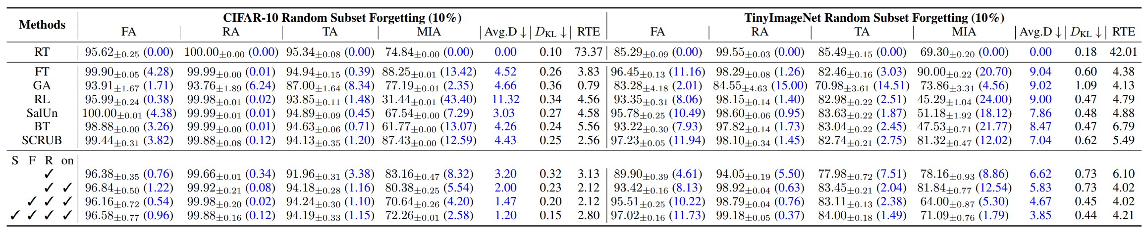
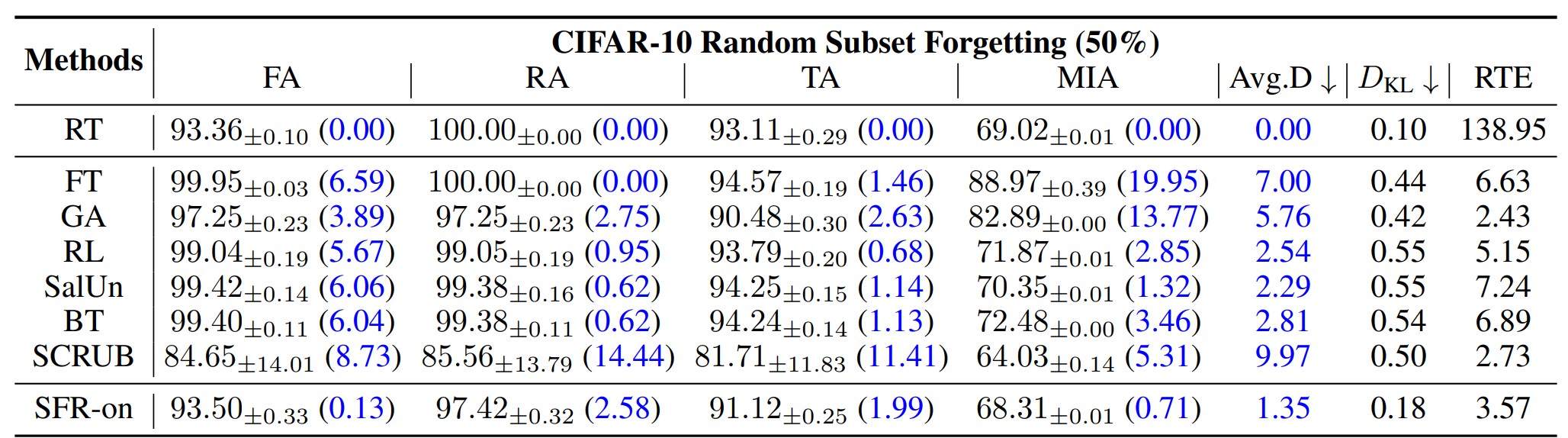
The above tables show the accuracy, KL divergence, and RTE (Run Time Efficiency) of each unlearning model in the classification task when forgetting 10% and 50% of the total dataset, respectively. The accuracy and KL divergence measurement results confirm that SFR-on produced results closest to the retraining method.
Furthermore, these results also allow us to measure the contribution of each element (S, F, R-on) of SFR-on to the model. As a result, the model incorporating all three elements performs the best, but if there were additional results measuring only the individual contribution of each S, F, and R-on element to model performance, the impact of each element could be understood more objectively.
SFR-on in the Image Generation Task
Since applying the retraining approach to image generation models is difficult, the paper defines a new retraining method and compares it with existing approaches. As a result, it can be confirmed that SFR-on showed the smallest difference in accuracy and KL divergence results.
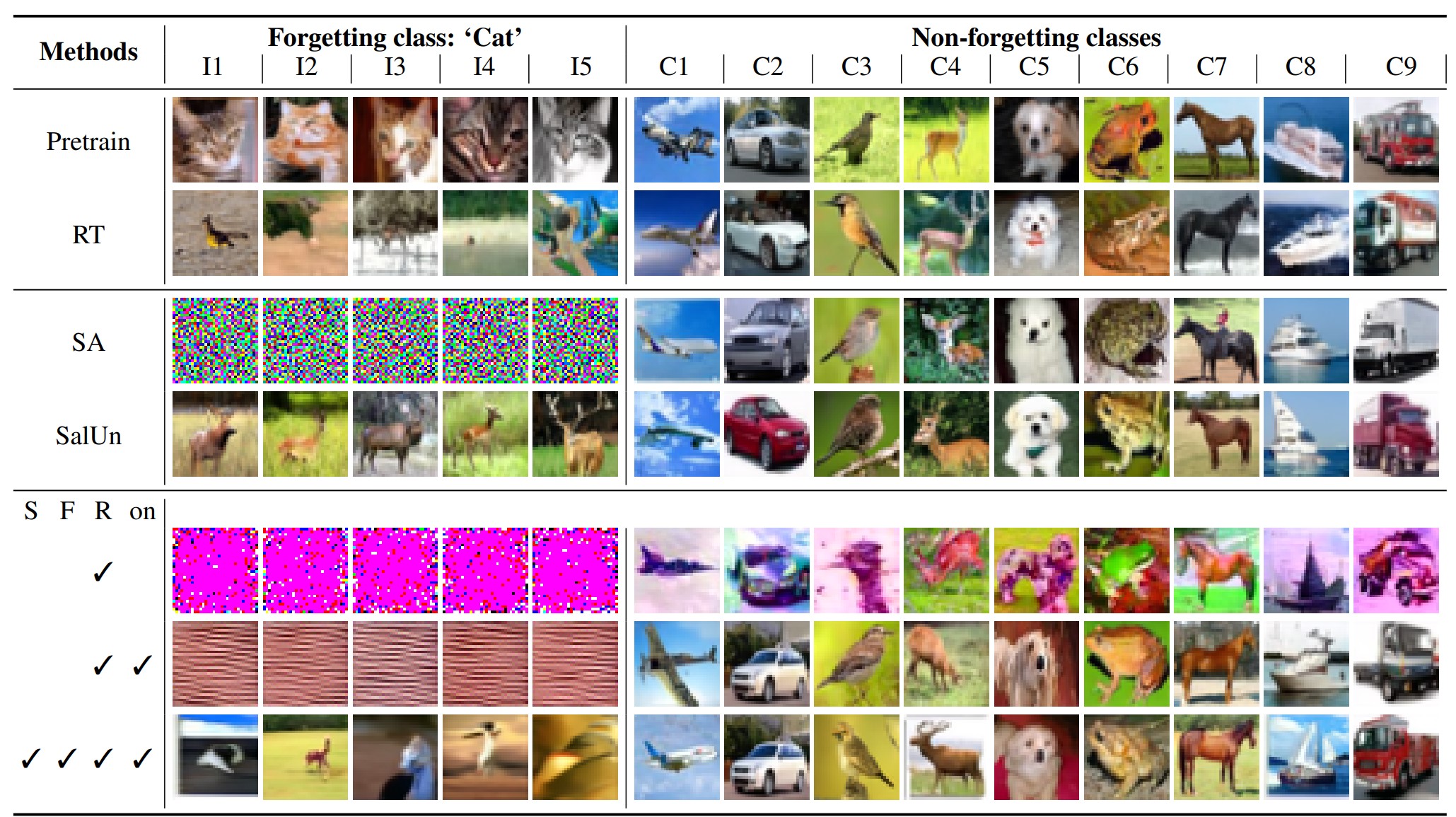
Additionally, the image generation performance when a specific concept has been forgotten can also be observed.
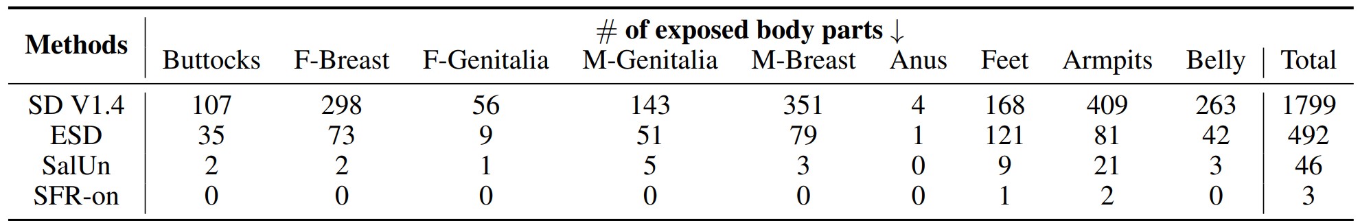
When entering related concepts as prompts in a model that has forgotten the NSFW concept, it can be confirmed that SFR-on generates the fewest related images compared to other unlearning techniques.