Paper: Adversarial Examples in the Physical World
Authors: Alexey Kurakin, Ian J. Goodfellow, Samy Bengio
Venue: ICLR 2017 Workshop Track
Introduction
Adversarial examples are inputs that have been subtly modified—almost imperceptibly to humans—yet deliberately alter the predictions of deep learning models. Prior research has primarily addressed adversarial examples in the digital domain, assuming the attacker can directly inject inputs into the model and that pixel-level manipulations are faithfully transmitted.
However, real-world systems are far more complex. Many models—such as camera-based image classifiers, autonomous driving perception systems, mobile apps, and video surveillance systems—observe physical-world objects through sensors before classification. In such cases, the attacker’s crafted input undergoes printing, photographing, lighting changes, distance variations, angle changes, sensor noise, compression, and other transformations that alter it from the original. Therefore, whether adversarial examples crafted in the digital domain survive in the physical world requires separate verification.
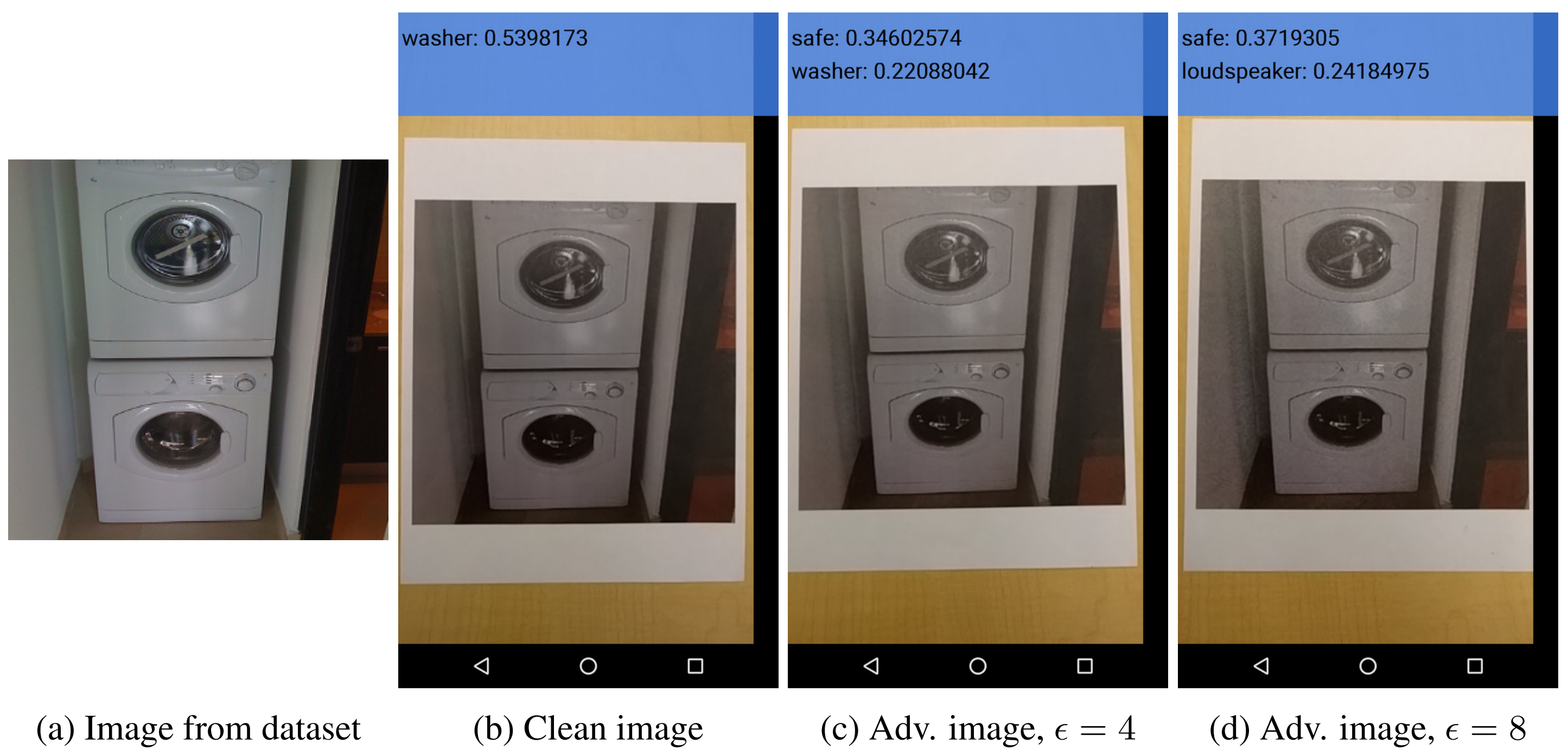
This paper generates adversarial images targeting an ImageNet Inception v3 classifier, prints them out, re-photographs them with a cellphone camera, and tests whether the results still cause misclassification. The key finding is that a substantial number of adversarial examples remain effective even after physical transformation.
The paper also compares which generation methods are more robust to physical transformations, and analyzes the print-and-photograph process through artificial transformations such as brightness, contrast, blur, noise, and JPEG compression. These findings suggest that adversarial attacks can pose a real threat in the physical world.
Background
Adversarial Examples
An adversarial example is an input \(X_{adv}\) created by adding a small perturbation to a normal input \(X\). It appears nearly identical to humans, but causes the model to misclassify it.
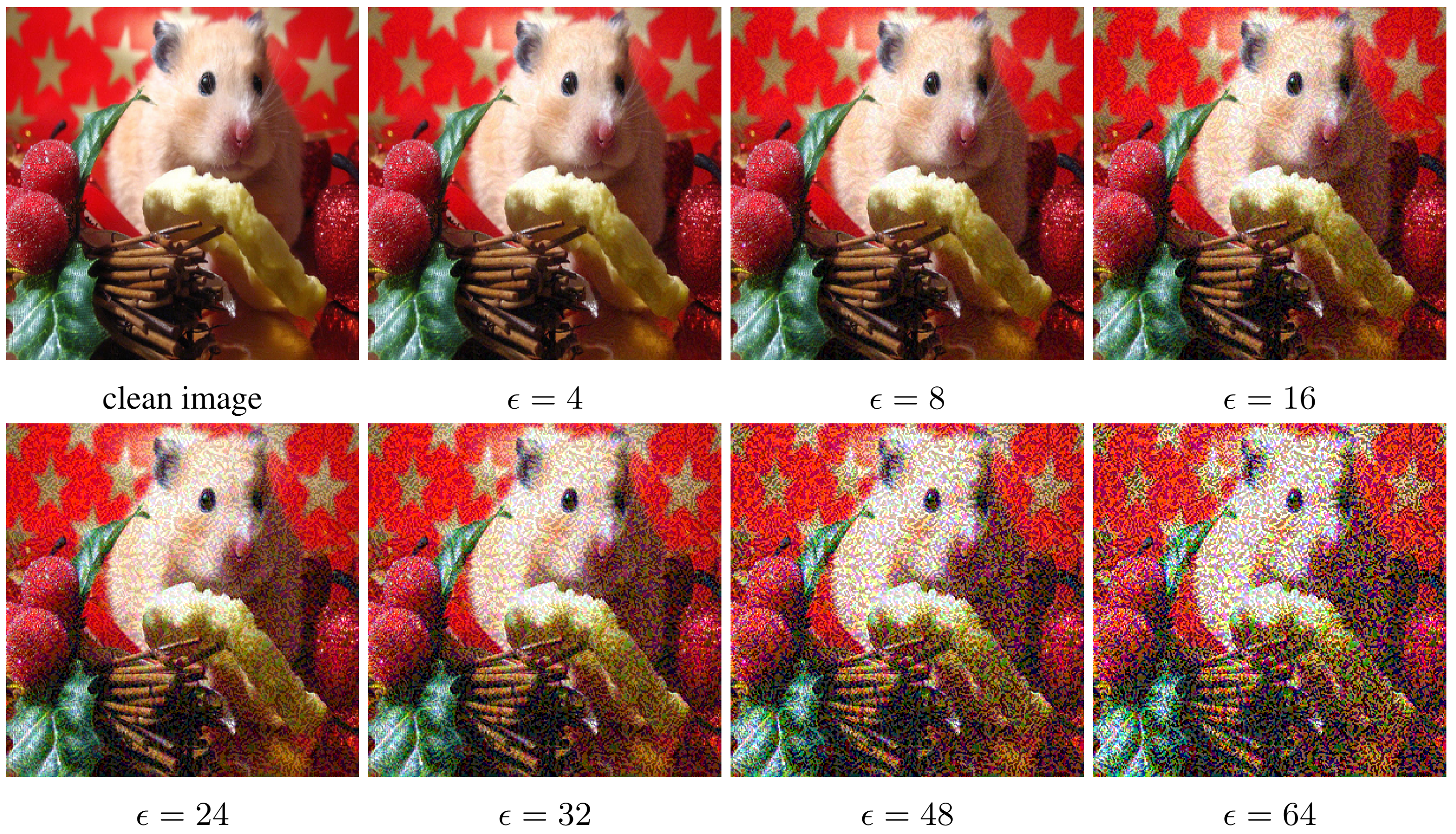
This paper uses an \(L_{\infty}\) constraint to ensure pixel values do not change significantly. Specifically, each pixel’s change is limited to at most \(\epsilon\). Smaller \(\epsilon\) values appear more natural to the human eye, but the attack strength may be weaker.
Notation
| Symbol | Meaning |
|---|---|
| \(X\) | Original image |
| \(y_{true}\) | True class of the original image |
| \(J(X, y)\) | Cross-entropy loss for input \(X\) and class \(y\) |
| \(X_{adv}\) | Adversarial image |
| \(\epsilon\) | Maximum allowed pixel perturbation magnitude |
| \(Clip_{X,\epsilon}\{X'\}\) | Operation that clips \(X'\) within the \(L_{\infty}\)-ball of radius \(\epsilon\) around \(X\) |
Adversarial Example Generation Methods
The paper compares three generation methods.
| Method | Key Idea | Characteristics |
|---|---|---|
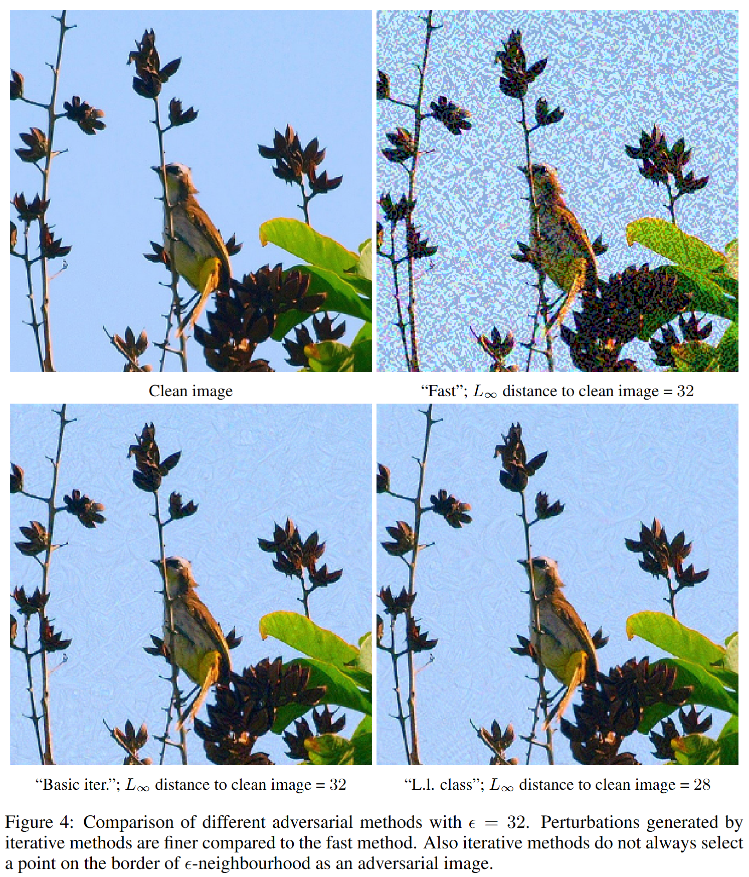
| Fast method | One-step move in the direction that maximally increases the loss | Fast but produces coarse perturbations |
| Basic iterative method | Multiple small-step iterations | Generates more refined perturbations |
| Iterative least-likely class method | Guides toward the class the model considers least likely | Strongly targeted, induces more dramatic misclassifications |
Fast Method
The fast method linearly approximates the loss function in the neighborhood of the input, then takes a single step in the sign direction that maximally increases the loss. This is equivalent to the FGSM formulation.
\[X_{adv} = X + \epsilon \cdot \operatorname{sign}(\nabla_X J(X, y_{true}))\]This method can generate an attack sample with just one backward pass, making it computationally very cheap. However, the perturbation is relatively coarse and may be less effective than iterative methods in the digital domain.
Basic Iterative Method
The basic iterative method repeatedly applies the fast method with a small step size.
\[X^{adv}_{0} = X\] \[X^{adv}_{N+1} = Clip_{X,\epsilon} \left\{ X^{adv}_{N} + \alpha \cdot \operatorname{sign}(\nabla_X J(X^{adv}_{N}, y_{true})) \right\}\]The paper uses \(\alpha = 1\), changing each pixel by at most 1 per step. The number of iterations is determined empirically. This approach can exploit the classification boundary with finer perturbations, often producing stronger attacks in the digital domain.
Iterative Least-Likely Class Method
The two methods above are non-targeted attacks that simply aim to break the correct classification. In contrast, this method is a targeted iterative attack that selects the class \(y_{LL}\) (Least Likely class) the model considers least probable and pushes the input toward it.
\[y_{LL} = \arg\min_{y} p(y|X)\] \[X^{adv}_{N+1} = Clip_{X,\epsilon} \left\{ X^{adv}_{N} - \alpha \cdot \operatorname{sign}(\nabla_X J(X^{adv}_{N}, y_{LL})) \right\}\]This approach can induce more dramatic misclassifications, such as making a dog be classified as an airplane. However, such refined perturbations may be more vulnerable to physical transformations.
Adversarial Example Generation Experiments
Objective
Before conducting physical-world experiments, the paper compares how effective the three attack methods are in the digital domain. The purpose of this stage is to determine how well each attack fools the original model, and at what range of \(\epsilon\) a meaningful attack can be achieved with only “small noise”-level perturbations.
Experimental Setup
- Dataset: ImageNet validation set, 50,000 images
- Model: Pre-trained Inception v3
- Attack methods: fast, basic iterative, iterative least-likely class
- Perturbation magnitude: \(\epsilon = 2 \sim 128\)
- Evaluation metrics: top-1 accuracy, top-5 accuracy
Using the accuracy on clean images as the baseline, the accuracy of adversarial images is measured for each attack method and \(\epsilon\) combination. Top-1 accuracy is the proportion of cases where the model’s top prediction matches the ground truth, and top-5 accuracy is the proportion where the correct class appears among the top 5 predictions.
Experimental Results
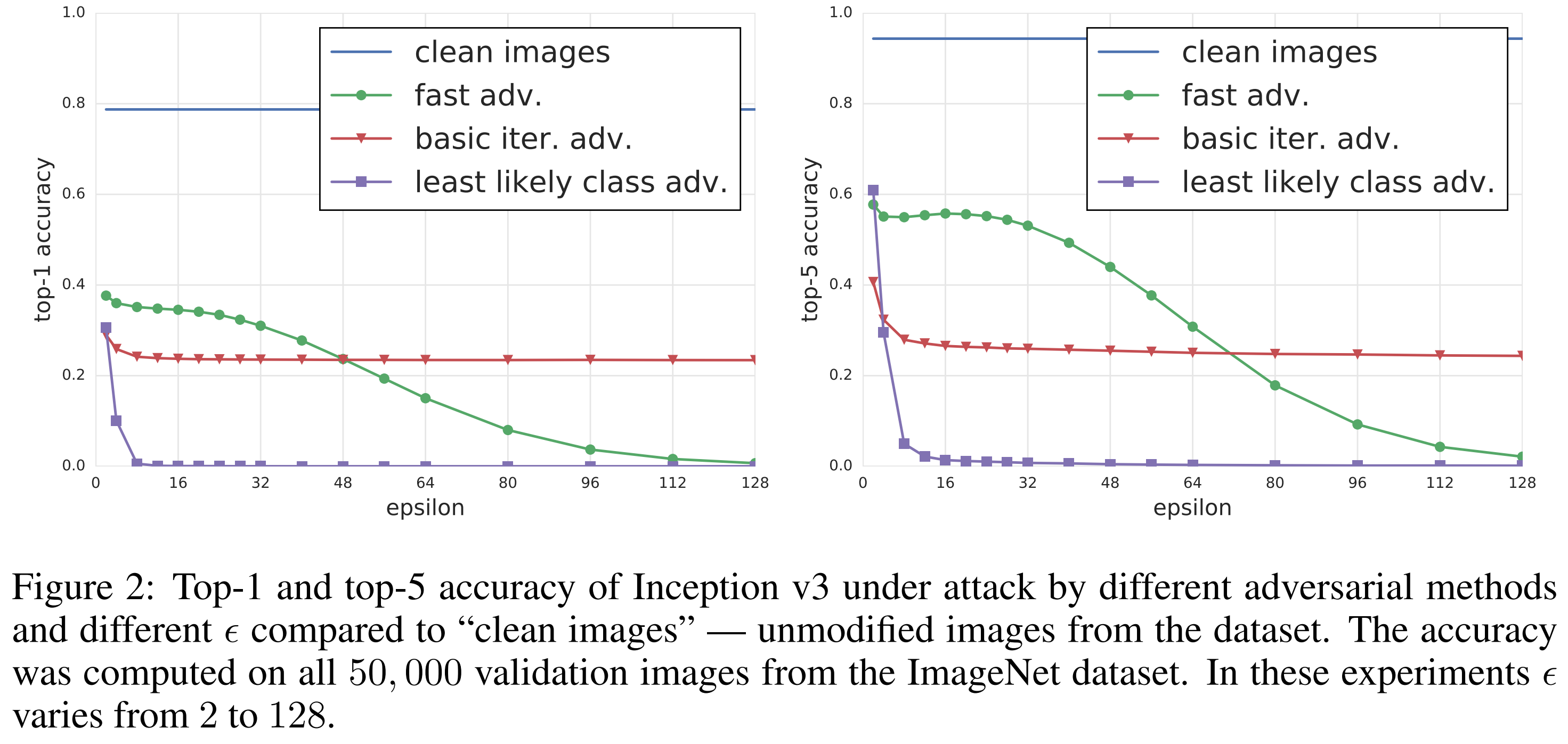
The results show that all three attack methods significantly degraded ImageNet classification performance.
First, the fast method, despite being the simplest approach, showed strong effects even at small \(\epsilon\) values. According to the paper, even at the smallest \(\epsilon\), it reduced top-1 accuracy to roughly half, and decreased top-5 accuracy by about 40%. However, when \(\epsilon\) becomes too large, the image itself begins to appear visibly degraded to humans.
In contrast, the iterative methods use finer perturbations, allowing them to induce higher misclassification rates while relatively preserving image content. In particular, the least-likely class method was found to effectively cause misclassification even at smaller \(\epsilon\) values.
The paper restricts all subsequent physical-world experiments to \(\epsilon \le 16\). The reason is that perturbations in this range still appear as minor noise to humans while sufficiently confusing the classifier. In other words, what matters is that the attacks demonstrated in the physical experiments are not “visibly corrupted images” but rather show that “attacks are possible even on relatively natural-looking images.”
Physical-World Experiments
Destruction Rate
To evaluate how well adversarial examples retain their adversarial properties after physical transformation, the paper defines a metric called the Destruction rate \((d)\). This is the proportion of adversarial examples that were successful in the digital domain but fail after transformation. A lower destruction rate means adversarial examples survive well after transformation, while a higher rate means the physical transformation effectively neutralizes the attack.
\[d = \frac{ \sum_{k=1}^{n} C(X_k, y_k^{true}) \overline{C}(X_k^{adv}, y_k^{true}) C(T(X_k^{adv}), y_k^{true}) }{ \sum_{k=1}^{n} C(X_k, y_k^{true}) \overline{C}(X_k^{adv}, y_k^{true}) }\]| Symbol / Expression | Description |
|---|---|
| $T(\cdot)$ | Transformations occurring in the physical environment, such as printing and re-photographing |
| $C(X,y)$ | Function that returns 1 if image $X$ is correctly classified as class $y$, 0 otherwise |
| $\overline{C}(X, y) = 1 - C(X, y)$ | Indicator function denoting whether the model misclassifies |
Experimental Setup
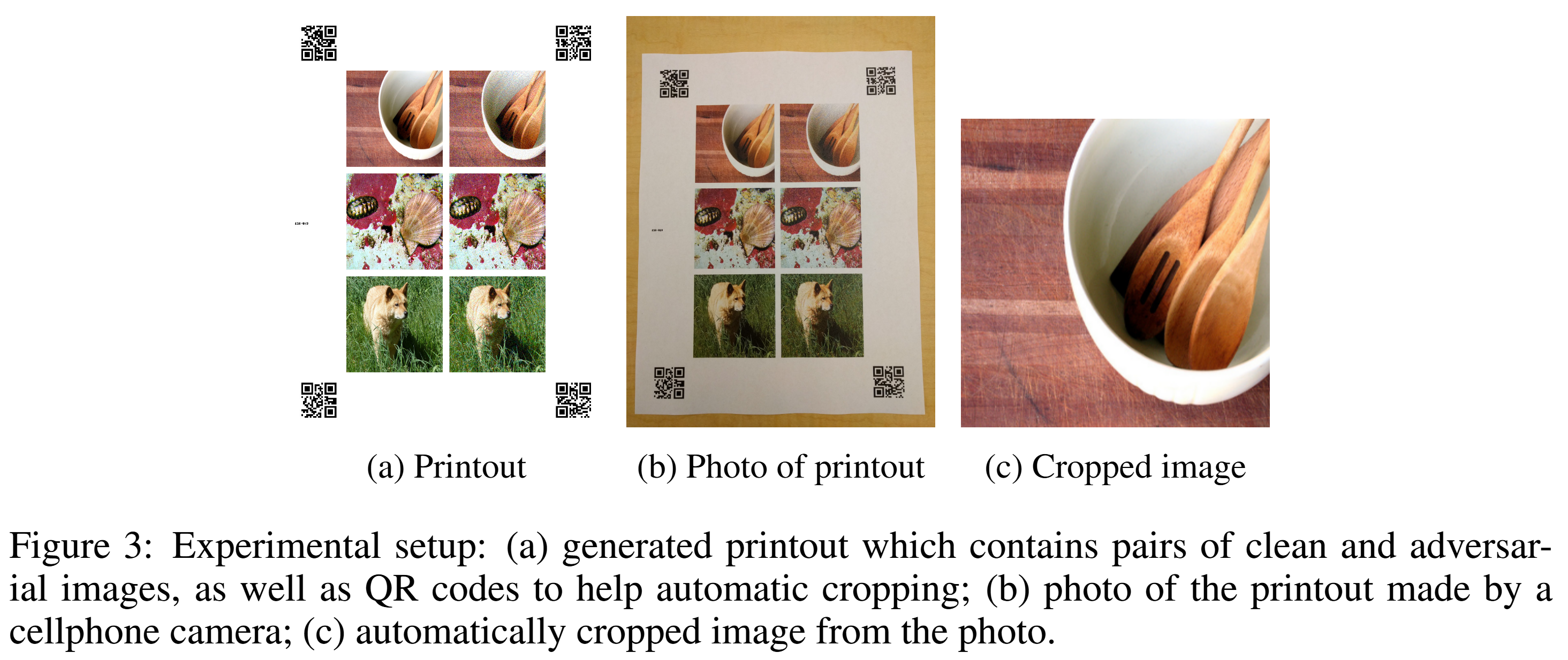
The pipeline for the physical-world experiments is as follows:
- Print digital clean images and adversarial images.
- Photograph the printouts with a cellphone camera.
- Automatically crop and warp the original examples from the photographs.
- Feed them back into the classifier and measure accuracy and destruction rate.
The detailed settings are as follows:
- Printing device: Ricoh MP C5503 office printer, 600 dpi
- Camera device: Nexus 5x cellphone camera
- Preprocessing: QR codes placed at printout corners for automatic detection and cropping
- Photo environment: Standard indoor lighting, without strict control over camera angle and distance
The authors intentionally did not fully control lighting, distance, angle, etc. This was to preserve some realistic nuisance variability—the design was intended to observe how much real-world distortions degrade adversarial perturbations.
Average Case and Prefiltered Case
The paper evaluates physical attacks under two scenarios:
- Average case: Adversarial examples are generated and attacks are performed on 102 randomly selected images.
- Prefiltered case: To test more aggressive adversarial examples, images are selected based on the following criteria: 102 images where clean images are correctly classified in the digital domain, while adversarial images are misclassified in both top-1 and top-5, with prediction confidence of 0.8 or higher.
The average case examines “how effective is an attack on arbitrary inputs in reality,” while the prefiltered case examines “how strong does the attack become when the attacker selects favorable samples.”
Physical-World Experiment Results
The results showed that a significant number of adversarial images still caused misclassification even after printing and photographing. In other words, physical transformation weakens the attack but does not completely neutralize it.
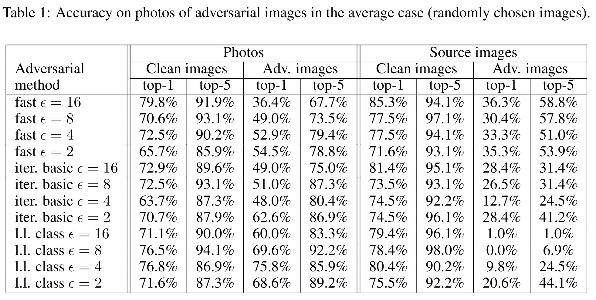
The table above shows the accuracy for the average case. For fast method with \(\epsilon = 16\), the top-1 accuracy of photographed adversarial images was 36.4%. In other words, approximately 63.6% still caused top-1 misclassification. The top-5 accuracy was 67.7%, meaning about 32.3% of attacks were still effective even by the top-5 criterion.
An interesting finding is that the fast method was more robust to physical transformations than the iterative methods. The top-1 destruction rates for the average case are as follows:
| Attack Method | Rate |
|---|---|
| fast $\epsilon = 16$ | 12.5% |
| basic iterative $\epsilon = 16$ | 40.4% |
| least-likely class $\epsilon = 16$ | 72.2% |
That is, iterative attacks that appeared stronger in the digital domain actually broke down more easily during the actual print-and-photograph process. The paper interprets this as iterative methods relying on finer and more delicate co-adaptation. The more refined the perturbation, the more easily it is damaged by small real-world distortions.
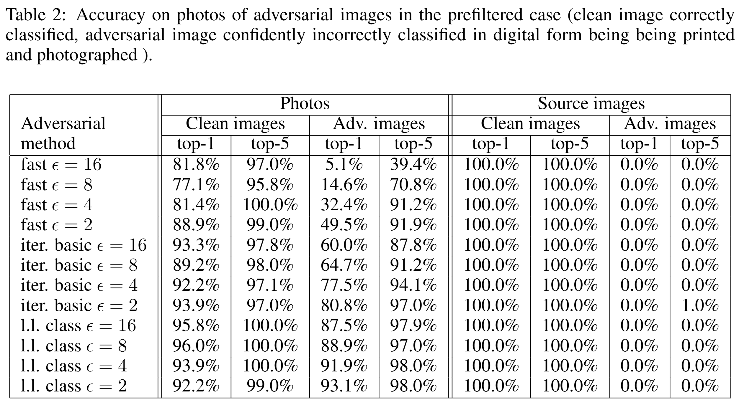
The table above shows the accuracy for the prefiltered case, and similar trends to the average case are observed. Even when attacking only pre-selected samples that were highly susceptible, physical transformation still dealt significant damage to iterative attacks.
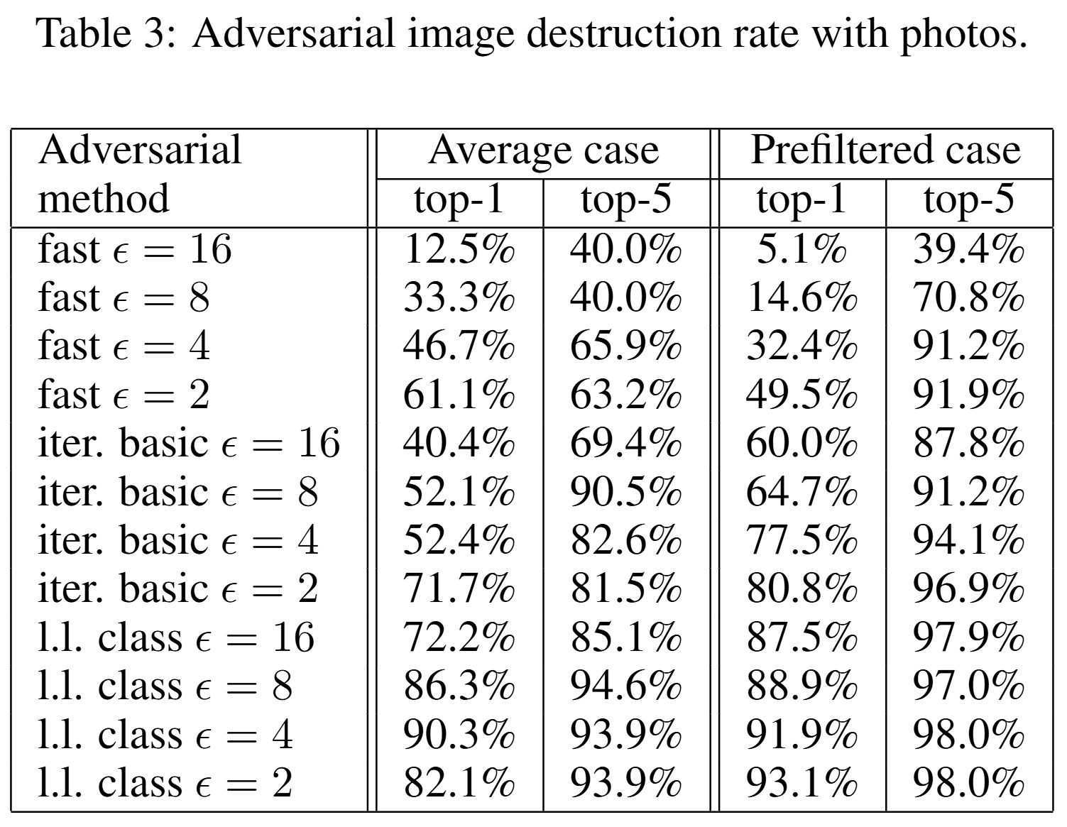
The table above shows the destruction rate results for both cases. This indicates whether adversarial examples generated in the digital domain lost their attack effectiveness in the physical world. There are instances where the prefiltered case destruction rate is higher than the average case, suggesting that attacks that are overly well-tuned in the digital domain may be more vulnerable to real-world transformations. In summary, adversarial attacks in the physical world are clearly possible, but which attack is more threatening cannot be judged solely by digital performance.
Physical-World Black-Box Attack
Although the main experiments were conducted in a white-box setting, the paper also demonstrates black-box attacks in the physical world. The authors showed adversarial printouts created targeting Inception v3 to the mobile TensorFlow Camera Demo app, and observed that clean images were correctly classified while adversarial images were misclassified. This result provides qualitative evidence that adversarial example transferability can work meaningfully in the physical world. It suggests that even when attackers do not know the internals of the target model, adversarial examples crafted from a surrogate model may still be effective against real camera-based systems.
Artificial Image Transformation Experiments
Objective
The print-and-photograph process is a highly composite transformation. To better understand this composite transformation, the paper decomposes the photography process into several controllable, simple artificial transformations and analyzes how adversarial examples are destroyed. Specifically, the complex real-world distortions are broken down into individual factors such as brightness, contrast, noise, and compression, and the contribution of each factor to destroying the adversarial properties is measured.
Experimental Setup
- Data: 1,000 randomly sampled images from the ImageNet validation set
- Transformation types: brightness/contrast changes, Gaussian blur, Gaussian noise, JPEG encoding
- Method: Apply transformations to adversarial images and measure the destruction rate
Experimental Results
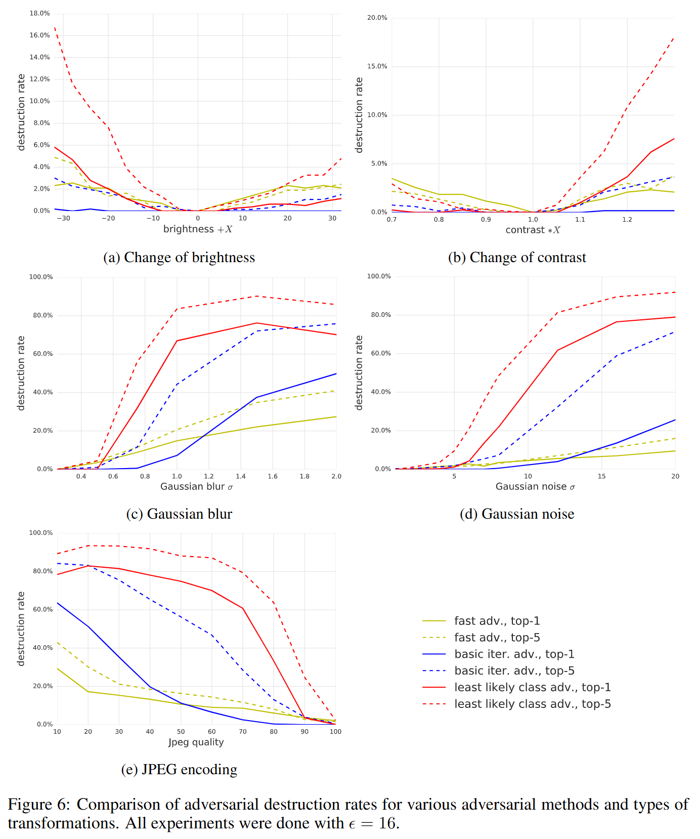
According to the graphs above, the effects of artificial transformations on adversarial examples are as follows:
-
(a) Change of brightness & (b) Change of contrast
- Changes in brightness or contrast result in very low destruction rates (generally below 20%).
- This means adversarial examples are not easily neutralized by simple brightness changes.
-
(c) Gaussian blur & (d) Gaussian noise
- Blurring or adding noise to images causes the destruction rate to rise sharply.
- In particular, sophisticated iterative attack methods like least-likely class, which rely on fine pixel adjustments, are very vulnerable to coarse transformations like blur and noise (destruction rates reaching 80-90%).
-
(e) JPEG encoding
- As JPEG compression strength increases (i.e., quality value decreases), the destruction rate rises.
- This is because the lossy compression process removes the subtle signals embedded for adversarial attacks.
Conclusion
This paper is a pioneering study that experimentally demonstrates that adversarial examples are not merely a mathematical or artificial phenomenon confined to the digital domain, but a real and viable threat in the physical world. The key messages of the paper can be summarized in three points:
- Threat persistence in physical environments: Adversarial images generated in the digital domain still cause model misclassification with a significant probability even after undergoing physical transformations such as printing and camera re-photographing.
- The paradox between attack sophistication and physical robustness: The most sophisticated and powerful attacks in the digital domain (e.g., least-likely class) are not always the most lethal in the physical world. Rather, relatively simple single-step attacks like the fast method exhibit greater resilience to physical transformations.
- Limitations of defense through simple transformations: Simple changes in brightness or contrast alone are insufficient to neutralize adversarial attacks. Coarser transformations such as blur, noise, and JPEG compression can somewhat reduce attack success rates, but they do not completely block the threat as a defense mechanism.
In conclusion, the greatest significance of this study lies in presenting the paradigm that when evaluating a model’s adversarial robustness, one must comprehensively consider not only the algorithmic vulnerabilities within the model itself, but the entire physical delivery path including sensors, printing, photographing, and compression.