Paper: Explaining and Harnessing Adversarial Examples
Authors: Ian J. Goodfellow, Jonathon Shlens & Christian Szegedy
Venue: In International Conference on Learning Representations (ICLR), 2015
Introduction
The Mystery of Adversarial Examples
Many machine learning models and state-of-the-art neural networks possess a critical weakness: they are highly vulnerable to adversarial examples. Adversarial examples are data created by taking a correctly sampled input from the original data distribution and adding a perturbation that is imperceptible to the human eye yet intentionally computed under a worst-case assumption. Remarkably, models produce completely incorrect predictions with very high confidence from such subtle changes alone.
Early researchers speculated that this phenomenon was caused by the extreme nonlinearity of deep neural networks and overfitting due to insufficient regularization in supervised learning.
However, this paper proves that such speculation is wrong. Instead, it argues that the fundamental reason neural networks are vulnerable to adversarial perturbations is that models are too linear. This linear perspective perfectly explains why adversarial examples generalize across diverse architectures and training datasets.
The Linear Explanation of Adversarial Examples
Linearity in High-Dimensional Spaces
Digital images often use 8 bits per pixel, so information below 1/255 of the dynamic range is discarded. Since the precision of the model’s input features is limited, if every element of a perturbation is smaller than the feature precision, the classifier should not respond differently to the original input and the adversarial input.
Consider a linear model as an example. The dot product of a weight vector $w$ and an adversarial example $\tilde{x}$ is as follows:
\[w^{\top}\tilde{x} = w^{\top}x + w^{\top}\eta\]The adversarial perturbation increases the activation by $w^{\top}\eta$. To maximize this increase under a max-norm constraint, one can simply set $\eta = sign(w)$. In high-dimensional problems, even a very small change along each input dimension accumulates linearly along the weight dimensions, producing a single massive change in the output. This demonstrates that linear behavior, rather than nonlinearity, is sufficient to generate adversarial examples.
A Fast and Efficient Attack: FGSM (Fast Gradient Sign Method)
Linear Perturbation Against Nonlinear Models
Modern neural network architectures such as LSTMs, ReLU networks, and Maxout networks are intentionally designed to behave linearly in order to facilitate optimization. Even nonlinear models like sigmoid networks are tuned to operate primarily in their non-saturated, linear regime.
Because of this property, cheap and analytical perturbation methods that exploit linear models can inflict equally severe damage on neural networks. The authors propose the Fast Gradient Sign Method (FGSM), which computes the optimal adversarial perturbation by linearizing the cost function around the current parameters.
\[\eta = \epsilon sign(\nabla_{x}J(\theta,x,y))\]The required gradient can be computed very efficiently using backpropagation.
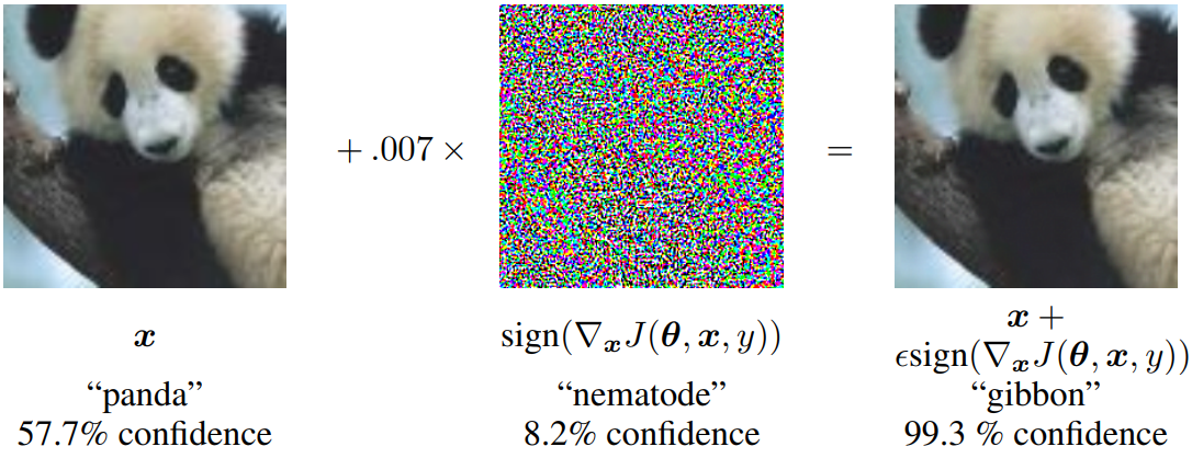
In practice, when a perturbation of a certain magnitude was applied using this method, a shallow softmax classifier recorded a 99.9% error rate on the MNIST test set, and a Maxout network exhibited an 89.4% error rate.
Improving Model Robustness: Adversarial Training
A New Regularization Technique
Unlike shallow linear models, deep networks possess the capacity to represent functions that can at least resist adversarial perturbations. According to the universal approximator theorem, a network with a sufficient number of hidden units can approximate any function. The problem is that standard supervised training does not inherently encourage the model to learn resistance against adversarial examples.
Therefore, a method was proposed that directly integrates an FGSM-based adversarial objective function into the training process.
\[\tilde{J}(\theta,x,y) = \alpha J(\theta, x, y) + (1-\alpha)J(\theta, x + \epsilon sign(\nabla_{x}J(\theta,x,y)))\]The paper used $\alpha=0.5$ in its experiments. By continuously updating the supply of adversarial examples during training, this approach successfully reduced the error rate of a Maxout network with dropout from 0.94% to 0.84%, demonstrating an excellent regularization effect. The model’s error rate on adversarial examples also dropped dramatically from 89.4% to 17.9%.
Why Do Adversarial Examples Generalize?
Transferability Across Models
One of the most intriguing properties of adversarial examples is that examples crafted to fool a specific model can also fool other models with entirely different architectures or training data. Moreover, the misclassified classes often agree across models. If extreme nonlinearity or overfitting were the cause, it would be impossible to explain why different models produce the same incorrect predictions for the same example.
From the linear perspective, adversarial examples do not exist in fine pockets scattered densely throughout space like rational numbers, but rather occur across broad subspaces. In other words, one can reliably generate adversarial examples simply by scaling the perturbation sufficiently in the correct direction – one that has a positive dot product with the gradient of the cost function. Since machine learning algorithms learn similar classification weights by generalizing from the same dataset, the stability of the weights directly translates to the stability (transferability) of adversarial examples.
Conclusion
Key Summary and the Paradox of Optimization
The main results running through this paper are as follows:
- Adversarial examples are a property of high-dimensional dot products, arising from linearity rather than nonlinearity.
- Adversarial examples generalize across different models because perturbations are strongly aligned with the model’s weight vectors, and different models learn similar functions.
- The direction of the perturbation matters most, not the specific point in space.
- Models that are easy to optimize are easy to perturb.
Consequently, state-of-the-art AI models can perfectly classify training data but harbor a serious flaw: they make incorrect predictions with excessively high confidence in regions outside the data distribution. The “ease of optimization” adopted by deep learning comes at the cost of models that can be easily misled.
This study demonstrated that adversarial training can partially mitigate these flaws and raises an important implication: the development of robust optimization techniques that can guarantee locally more stable behavior is needed in the future.