Paper: Intriguing Properties of Neural Networks
Authors: Christian Szegedy, Wojciech Zaremba, Ilya Sutskever, Joan Bruna, Dumitru Erhan, Ian Goodfellow, and Rob Fergus
Venue: In International Conference on Learning Representations (ICLR), 2014
Introduction
Deep neural networks are powerful models that achieve outstanding performance in tasks such as visual and speech recognition. However, it is extremely difficult for humans to interpret the reasoning behind the computational results automatically learned through backpropagation, and these networks even possess properties that contradict our general intuition. This paper experimentally identifies two counter-intuitive properties of deep neural networks.
The first property is that individual units do not encode specific semantic meaning; instead, information is distributed in a complex manner across the space of activations. Here, “semantic meaning” refers not to raw pixel values but to the actual meaning that humans perceive visually. For example, our general intuition suggests that in a model classifying animals, a specific neuron would be dedicated to detecting a dog’s ear while another neuron would detect a dog’s nose. However, the paper demonstrates through experiments that this intuition is entirely wrong, proving the counter-intuitive property that meaningful concepts can be found equally well along arbitrary random directions, not just along individual unit axes.
The second property is that deep neural networks do not possess robust stability against small perturbations applied to input data. Intuitively, we would expect that if noise so subtle that humans cannot even perceive it is added, the model’s prediction should remain unchanged. However, experimental results in the paper revealed that adding imperceptibly small noise to pixel values is sufficient to manipulate the model into producing completely wrong predictions. The manipulated data generated by adding such perturbations intended to deliberately fool the model’s predictions is defined in this paper as adversarial examples.
These properties suggest that even highly trained deep neural networks via backpropagation operate in a fundamentally different way from human perception and possess structurally inherent intrinsic blind spots.
Main Discussion
The Location of Semantic Meaning Learned by Neural Networks
Traditional computer vision techniques were highly intuitive. They relied on feature extraction based on human intuition, such as “color histograms” or “quantized local derivatives (techniques that record the direction of edges).” In simple terms, in the space where data resides, each axis was designed to carry specific semantic information: axis 1 represents “the amount of red,” axis 2 represents “the sharpness of a particular edge,” and so on. Because of this, even when examining a single coordinate of the feature space in isolation, it was easy to interpret and connect how meaningful changes in the actual image occurred as the value increased or decreased.
Previous researchers attempted to apply this intuition from traditional computer vision to neural networks. Specifically, they interpreted the activation value of a particular hidden unit as a meaningful single feature. To determine what meaning a specific neuron encodes, they searched for the images that most strongly activate that neuron using the following formula: \(x^{\prime} = \arg \max_{x \in \mathcal{I}} \langle \phi(x), e_i \rangle\)
- \(x\): input image
- \(\phi(x)\): activation values output from a specific hidden layer
- \(\mathcal{I}\): a held-out set of test images that the network has not seen during training
- \(e_i\): the natural basis vector corresponding to the \(i\)-th hidden unit
This formula describes the process of finding a specific image \(x^\prime\) within the image dataset \(\mathcal{I}\) that maximizes the activation value of the \(i\)-th neuron.
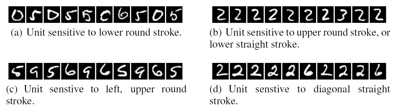
In experiments using the MNIST dataset, the images found in this way appeared to share consistent visual commonalities such as “a stroke with a rounded bottom” or “a diagonal straight line.”
The authors then conducted the same experiment using completely random directions (\(v\)) instead of individual units. The formula and its results are shown below.
\[x^{\prime} = \arg \max_{x \in \mathcal{I}} \langle \phi(x), v \rangle\]- \(v\): an arbitrary random direction vector within the activation space
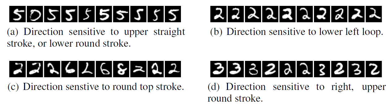
If, as previously believed, individual neurons were trained to carry specific meanings, then images maximizing a random direction (\(v\)) – an arbitrary mixture of multiple neurons – should show no commonalities whatsoever. However, even when collecting images that maximize activation values along random directions, clear and interpretable commonalities appeared, just as when examining individual neurons. These two experimental results prove that the meaningful information learned by neural networks is not partitioned into individual neurons but is broadly distributed across the entire activation space formed by the neurons.
Adversarial Examples
In general, deep neural networks possess non-local generalization ability due to the many nonlinear layers between the input and output.
Let us illustrate with an example. In a model that classifies cars, a front-view image and a side-view image of the same car are very far apart in terms of the pixel values received by the computer. However, as the deep learning model passes through its deep layers, it learns that these two images represent the same object and can predict both as “car.”
Furthermore, because of this non-local generalization ability, it was assumed that the model would also possess local generalization ability – being able to predict the correct answer with high probability even when imperceptibly small perturbations are added to the input image. However, experiments proved that when adversarial examples were created by adding small perturbations generated through a specific optimization algorithm to original images, the model completely misclassified them.
Let us first examine the formulation.
The authors defined the problem of applying very subtle manipulations (perturbations) to original images so that the model classifies them as a specific wrong label as a mathematical optimization problem. Given a specific image \(x\), the formula for finding the minimum noise \(r\) that causes model \(f\) to classify it as the target wrong label \(l\) is as follows:
\[\begin{aligned} & \text{Minimize } \|r\|_2 \text{ subject to:} \\ & 1.\ f(x + r) = l \\ & 2.\ x + r \in [0, 1]^m \end{aligned}\]Meaning of the Formulation
-
\(\|r\|_2\) minimization: Minimizing the L2-norm of the noise to generate noise small enough to be imperceptible to humans
-
\(x + r \in [0, 1]^m\): A constraint ensuring that pixel values do not exceed the valid representation range of an image due to the added noise
-
\(f(x + r) = l\): A constraint forcing the prediction result to be the intended wrong label when the manipulated image (\(x + r\)) is fed into the model
Since deep neural networks have nonlinearity and non-convex characteristics, finding an exact solution to the above formulation is practically infeasible. Therefore, the authors introduced the L-BFGS algorithm to transform the problem into an easier approximate form.
\[\text{Minimize } c|r| + \text{loss}_f(x + r, l) \quad \text{subject to } x + r \in [0, 1]^m\]This modified formulation means finding the optimal \(r\) by adjusting the constant \(c\) to suppress the magnitude of noise added to the image as much as possible while also minimizing the loss that drives the model to classify as the target wrong answer.
Using this formulation, the authors conducted experiments on models such as AlexNet and QuocNet.
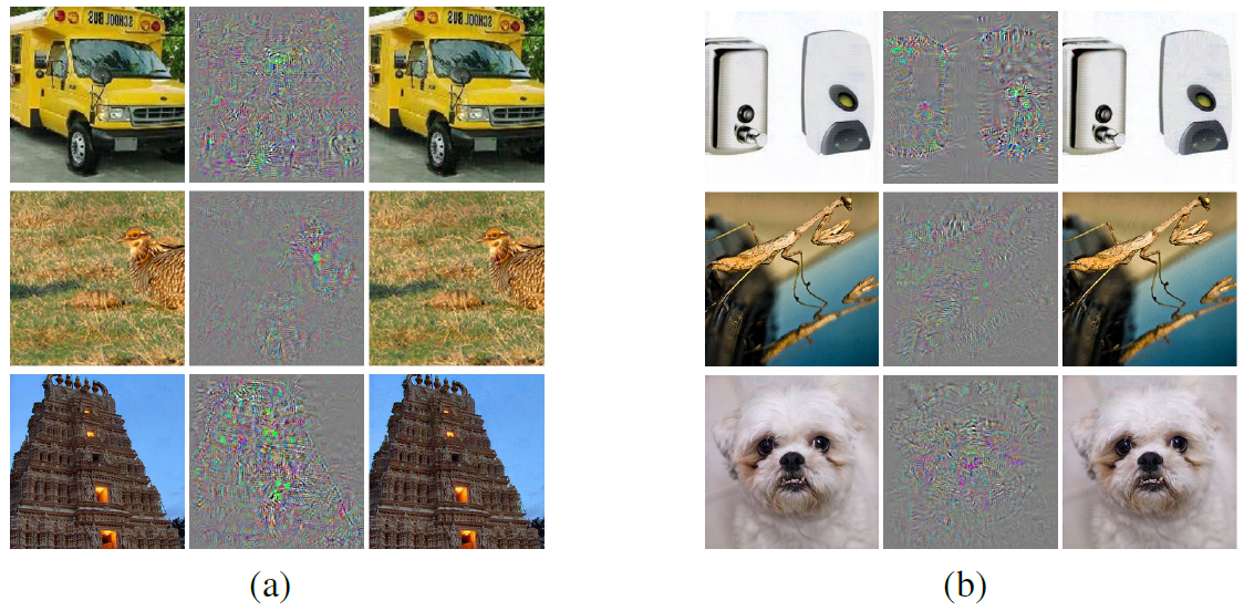
The figure above shows, from the left column, the original image correctly predicted, the applied noise, and the adversarial example created by adding the noise to the original image, respectively. The noise has been amplified 10x for visual clarity. After applying noise optimized to make the model confidently predict “ostrich,” even images that clearly belong to entirely different classes were misclassified as “ostrich.”
Generalization of Adversarial Examples
Subsequently, two experiments were conducted to test whether attacks using adversarial examples are not limited to a specific model but possess the ability to generalize.
The first experiment verified whether networks with completely different architectures and hyperparameters misclassify the same adversarial examples. The models used for the experiment and the results are as follows.
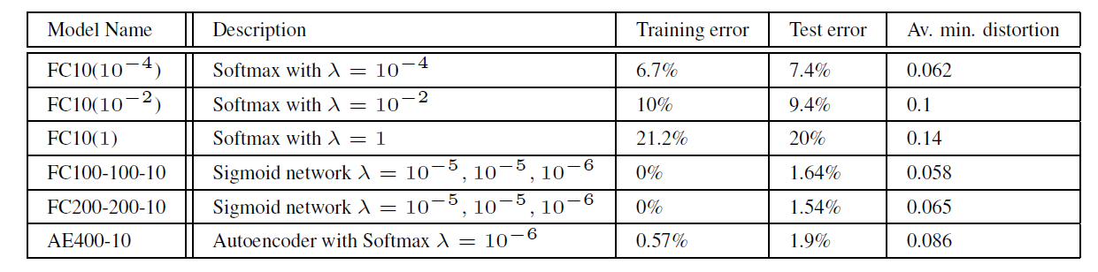
- \(\lambda\): the strength of weight decay
- Av. min. distortion: the minimum average pixel distortion that must be added to original images to collapse the model’s accuracy to 0%
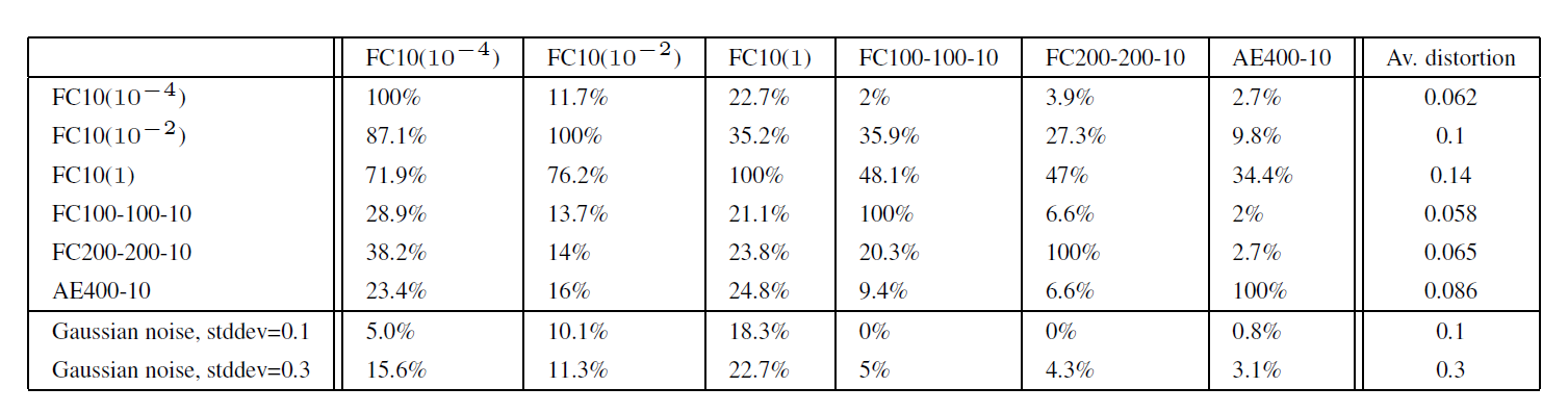
- Row: the model used to generate the adversarial noise (adversarial examples)
- Column: the model that receives and evaluates the images with the applied noise
The experimental results showed that noise crafted to fool a specific network caused misclassification at a significant rate even on models with entirely different architectures. This indicates that attacks using adversarial examples possess the ability to generalize.
The second experiment was conducted to verify the generalization ability across networks trained on different subsets of training data. The authors split the MNIST dataset into two groups and trained them independently, then tested whether the models were still fooled by the same adversarial examples.
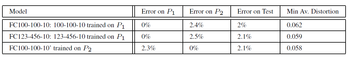
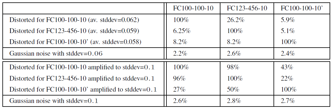
The experimental results confirmed that models trained on separate datasets misclassified each other’s adversarial examples.
These results suggest that adversarial examples are not the result of overfitting in a specific model but rather the result of intrinsic blind spots in the data distribution space that models learn.
Spectral Analysis of Instability
The authors mathematically analyzed how imperceptibly small noise can alter a model’s output. First, the output \(\phi(x)\) of a neural network with \(K\) layers is expressed as a composition of functions \(\phi_K\) from each layer. \(\phi(x) = \phi_K(\phi_{K-1}(\dots\phi_1(x; W_1); W_2)\dots; W_K)\)
The instability of the network can be measured by computing the upper Lipschitz constant of each layer. This represents the maximum amplification limit that noise can experience when passing through a specific layer. It is expressed mathematically as:
\[\forall x, r, \|\phi_k(x; W_k) - \phi_k(x + r; W_k)\| \le L_k \|r\|\]The upper bound on the total error at the final output is the product of the Lipschitz constants of all layers.
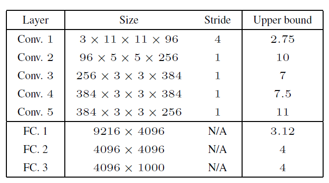
According to the paper, activation functions such as ReLU and Max-pooling have the property of contracting the differences in inputs. In contrast, weight matrices are the primary factor that amplifies differences in inputs. Mathematically, the Lipschitz constant \(L_k\) of a specific layer has its upper bound determined by the operator norm of that layer’s weight matrix \(W_k\) (the largest singular value, representing the maximum ratio by which the matrix can amplify its input). If the operator norm of each layer’s weight matrix is greater than 1, these values are continuously multiplied as the network deepens, ultimately causing noise to be amplified to large values at the output. The table below shows the computed upper bounds for each layer of the AlexNet model.
This mathematical analysis reveals the structural reason why deep learning models are inherently vulnerable to subtle manipulations.
Conclusion
This paper proved the counter-intuitive properties of deep neural networks through experiments and mathematical analysis. It also explains the distribution of adversarial examples by analogy to rational numbers. While the probability of adversarial examples occurring by chance is low, adversarial examples are densely scattered throughout the entire data space, just as rational numbers are densely packed between real numbers. Therefore, if we intentionally search for adversarial examples, we can find them sufficiently close to normal data.
The authors emphasize that a complete understanding of exactly how frequently adversarial examples appear in deep learning models and their fundamental cause is still lacking, and this is a key challenge that must be addressed in future research.