[NeurIPS🎉] Fantastic Robustness Measures: The Secrets of Robust Generalization

• 서론
• 사전 지식
  • 적대적 예제와 적대적 공격
  • 적대적 강건성과 적대적 방어
• 본론
• 결론
  • 관련 연구실 논문

서론

인공지능(Artificial Intelligence) 모델이 현실에 도입될 때에는 ‘대체로’ 잘 작동하는 것은 오히려 최소 조건이 됩니다. 오히려, 우리가 해당 모델을 신뢰할 수 있는지가 중요해집니다.

적대적 강건성(Adversarial Robustness)이란 “악의적인 공격자가 입력에 특정 노이즈(Noise)를 주었을 때에도 모델이 잘 작동할 수 있는가?”를 의미합니다. 현재 딥러닝(Deep Learning)을 포함한 인공지능 기술이 직면하고 있는 많은 결점들 중 가장 큰 결점이기도 합니다.

“Fantastic Robustness Measures: The Secrets of Robust Generalization” [Paper, Repo] 은 인공지능 최우수 학회인 NeurIPS 2023에서 발표된 본 연구실의 논문이며, 본 글에서는 기본적인 수학과 간단한 코드를 통해 적대적 강건성의 개념을 알아보고자 합니다.

사전 지식

적대적 예제와 적대적 공격

Source: https://adversarial-ml-tutorial.org/introduction/ [NeurIPS 2018 tutorial, “Adversarial Robustness: Theory and Practice”]

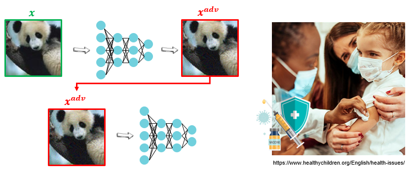
적대적 강건성을 가장 잘 이해하는 방법은 “적대적 예제를 만들어보는 것”입니다. 적대적 예제(Adversarial Example)이란 공격자가 정상적인 입력(Benign Input)에 악의적인 노이즈(Adversarial Noise)를 삽입한 것입니다. 이 때 사용되는 노이즈는 섭동(Perturbation)이라고도 불려집니다.

우선, PyTorch 내의 사전 훈련된 ResNet50 모델을 사용하여 정상적인(Benign) 돼지 사진을 분류해보겠습니다.

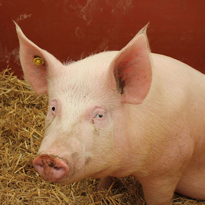
(1) 우선 사진을 읽어들이고 224x224로 사이즈를 변환합니다.

from PIL import Image
from torchvision import transforms

# read the image, resize to 224 and convert to PyTorch Tensor
pig_img = Image.open("pig.jpg")
preprocess = transforms.Compose([
   transforms.Resize(224),
   transforms.ToTensor(),
])
pig_tensor = preprocess(pig_img)[None,:,:,:]

# plot image (note that numpy using HWC whereas Pytorch user CHW, so we need to convert)
plt.imshow(pig_tensor[0].numpy().transpose(1,2,0))

(2) 크기가 조절된 이미지에 정규화(Normalization)을 거친 후, 학습된 ResNet50 모델을 불러와서 사진을 분류해보겠습니다.

import torch
import torch.nn as nn
from torchvision.models import resnet50

# simple Module to normalize an image
class Normalize(nn.Module):
    def __init__(self, mean, std):
        super(Normalize, self).__init__()
        self.mean = torch.Tensor(mean)
        self.std = torch.Tensor(std)
    def forward(self, x):
        return (x - self.mean.type_as(x)[None,:,None,None]) / self.std.type_as(x)[None,:,None,None]

# values are standard normalization for ImageNet images, 
# from https://github.com/pytorch/examples/blob/master/imagenet/main.py
norm = Normalize(mean=[0.485, 0.456, 0.406], std=[0.229, 0.224, 0.225])

# load pre-trained ResNet50, and put into evaluation mode (necessary to e.g. turn off batchnorm)
model = resnet50(pretrained=True)
model.eval()

# interpret the prediction
pred = model(norm(pig_tensor))

import json
with open("imagenet_class_index.json") as f:
    imagenet_classes = {int(i):x[1] for i,x in json.load(f).items()}
print(imagenet_classes[pred.max(dim=1)[1].item()])

hog

위 결과를 통해, 모델이 해당 사진은 돼지(“hog”)임을 정확히 맞춘 것을 확인할 수 있습니다. 모델이 정답을 잘 출력할 수 있는 이유는, 모델의 아래와 같은 학습 목표를 잘 달성했기 때문입니다.

\begin{equation} \label{eq:min} \min_\theta \ell(h_\theta(x), y) \end{equation}

이 때, \(h\)는 모델을 의미하며, \(\theta\)는 학습 대상이 되는 모델의 매개변수(parameter) 의미 합니다. \(h_\theta(x)\)와 \(y\) 사이의 차이를 정의하는 손실함수(loss function) \(\ell\)를 최소화하여, 우리는 모델이 특정 이미지 \(x\)에 대한 결과값인 \(h_\theta(x)\)와 정답인 \(y\)과 유사한 예측을 할 수 있도록 유도합니다.

적대적 예제는 “모델을 속이기” 위해 고안된 개념입니다. 따라서, 적대적 예제는 위의 학습 목표를 저해하기 위해 최소화했던 손실함수를 역으로 최대화하는 데에 중점을 둡니다.

\begin{equation} \label{eq:max} \max_{\hat{x}} \ell(h_\theta(\hat{x}), y) \end{equation}

위 식은 \(\ell(h_\theta(\hat{x}), y)\)을 최대화하는 새로운 이미지인 \(\hat{x}\)를 찾는 것을 목표로 합니다. 본 과정을 거쳐 생성된 이미지 혹은 예제를 적대적 예제(adversarial example)라고 부르게 됩니다.

나아가, 악의적인 사용자는 사람이 보기에는 돼지이지만, 딥러닝 모델은 돼지가 아니라고 하는 예제를 만드는 것이 목표입니다. 따라서, 적대적 예제 \(\hat{x}=x+\delta\)를 만들 때 더해지는 노이즈 \(\delta\)는 사람이 눈치채지 못하는 크기를 가지도록 제한됩니다.

\begin{equation} \label{eq:max2} \max_{\delta\in\Delta} \ell(h_\theta(x+\delta), y) \end{equation}

본 조건 하에 구해진 노이즈 \(\delta\)를 적대적 섭동(adversarial perturbation) 혹은 적대적 노이즈(adversarial noise)라고 부르게 됩니다.

위를 Pytorch로 구현한다면 아래와 같습니다.

import torch.optim as optim
epsilon = 2./255

delta = torch.zeros_like(pig_tensor, requires_grad=True)
opt = optim.SGD([delta], lr=1e-1)

for t in range(30):
    pred = model(norm(pig_tensor + delta))   # 섭동(노이즈) 추가 후 예측
    loss = -nn.CrossEntropyLoss()(pred, torch.LongTensor([341]))  # 손실값 계산
    if t % 5 == 0:
        print(t, loss.item())
    
    opt.zero_grad()
    loss.backward()  # 손실함수 최대화 (9번의 손실값에 -가 곱해졌으므로)
    opt.step()
    delta.data.clamp_(-epsilon, epsilon)  # 크기 제한
    
print("True class probability:", nn.Softmax(dim=1)(pred)[0,341].item())

0 -0.0038814544677734375
5 -0.00693511962890625
10 -0.015821456909179688
15 -0.08086681365966797
20 -12.229072570800781
25 -14.300384521484375
True class probability: 1.4027455108589493e-06

위 돼지 이미지는 사람의 눈에는 틀림없이 돼지이지만, 모델의 눈에는 아래와 같이 99%의 확률로 웜뱃(wombat)이라는 다른 동물로 분류됩니다.

Predicted class:  wombat
Predicted probability: 0.9997960925102234

이를 응용하면, 모델이 우리가 원하는 답을 내놓도록하는 적대적 예제를 구할 수도 있습니다.

delta = torch.zeros_like(pig_tensor, requires_grad=True)
opt = optim.SGD([delta], lr=5e-3)

for t in range(100):
    pred = model(norm(pig_tensor + delta))
    loss = (-nn.CrossEntropyLoss()(pred, torch.LongTensor([341])) + 
            nn.CrossEntropyLoss()(pred, torch.LongTensor([404])))
    if t % 10 == 0:
        print(t, loss.item())
    
    opt.zero_grad()
    loss.backward()
    opt.step()
    delta.data.clamp_(-epsilon, epsilon)

0 24.00604820251465
10 -0.1628284454345703
20 -8.026773452758789
30 -15.677117347717285
40 -20.60370635986328
50 -24.99606704711914
60 -31.009849548339844
70 -34.80946350097656
80 -37.928680419921875
90 -40.32395553588867

max_class = pred.max(dim=1)[1].item()
print("Predicted class: ", imagenet_classes[max_class])
print("Predicted probability:", nn.Softmax(dim=1)(pred)[0,max_class].item())

Predicted class:  airliner
Predicted probability: 0.9679961204528809

이 외에도 다양한 적대적 예제를 생성해내는 다수의 적대적 공격 방법이 존재합니다. 자세한 사항은 torchattacks를 참고바랍니다.

적대적 강건성과 적대적 방어

2003년에 적대적 예제의 존재가 발견된 이후, 선행 논문들은 모델이 적대적 예제에 대해서도 정확한 결과를 낼 수 있는 방법을 고안해왔습니다. 적대적 강건성(Adversarial Robustness)은 ‘모델이 적대적 공격에도 얼마나 잘 버틸 수 있는지’를 수치화한 지표라고 할 수 있습니다. 나아가, 적대적 공격에 대한 강건성을 높이기 위한 방법을 적대적 방어(Adversarial Defense)라고 부르게 됩니다.

다양한 적대적 방어 기법들이 제안되었지만, 그 중에서도 활발하게 연구되고 있는 방어 기법은 적대적 학습(Adversarial Training)입니다. 적대적 학습이란 모델 학습 중에 적대적 예제를 맞추도록 학습하여 강건성을 높이는 방법입니다. 즉, 백신을 맞는 것과 유사한 원리가 되겠습니다.

이는 수학적으로 다음과 같은 min-max 문제가 됩니다.

\begin{equation} \min_{\theta} \max_{\hat{x}} \ell(h_\theta(\hat{x}), y) \end{equation}

위의 min-max 문제를 풀기 위해, 다양한 적대적 방어 기법(AT, TRADES, MART 등)이 제안되었으며, 비약적인 강건성 향상을 이루어냈습니다. 보다 최신 수치는 https://robustbench.github.io/를 참고 바랍니다.

본론

현재까지의 다양한 적대적 방어 기법들은 각자 다른 방식으로 높은 강건성을 달성해왔습니다. 그 과정에서, 선행 논문들은 “모델의 특정 특성(measure)이 좋으면, 강건성도 좋다”라는 전개 방식을 채택해오기도 했습니다. 특정 특성으로는 마진(margin), 경계면 두께(boundary thickness), 립시츠 계수(Lipschitz Value) 등이 거론되었습니다.

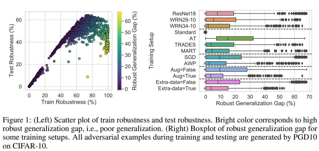
본 논문은 “과연 그러한 연구 가설들이 실험적으로도 검증될 수 있는가?”에 대한 고찰을 담고 있습니다. 선행 논문에서 자주 사용되는 8개의 학습 환경(모델 구조, 적대적 방어 기법, 배치 사이즈 등)을 고려하여 총 1,300개가 넘는 모델을 CIFAR-10 이미지 데이터에 대해 학습시켰습니다. 그리고, 각 모델의 특성들을 측정한 뒤, 해당 특성(measure)이 실제로 강건성(robustness)와 유의미한 관계를 갖는지 파악하였습니다.

본 논문에서는 강건성 값 자체보다도 해당 모델이 학습 데이터(training set)에 대한 강건성과 평가 데이터(test set)에 대한 강건성의 차이가 얼마나 작은지를 확인하기 위해 “강건성 일반화 차이(Robust generalization gap)”를 측정하였습니다. (※ 부록을 통해 강건성 값 자체를 측정하면 크게 유의미한 결과가 없음을 파악할 수 있습니다)

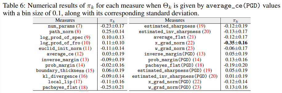
본 논문에서 제안된 평가 방법에 의한 확인 결과, 선행 연구에서 제안된 특성들 중 완벽히 강건성과 비례하는 특성은 존재하지 않았습니다. 특히, 적대적 방어 방법에 따라서도 편차가 큰 특성들이 많았으며, 대표적으로 경계면 두께(boundary thickness)가 그러하였습니다.

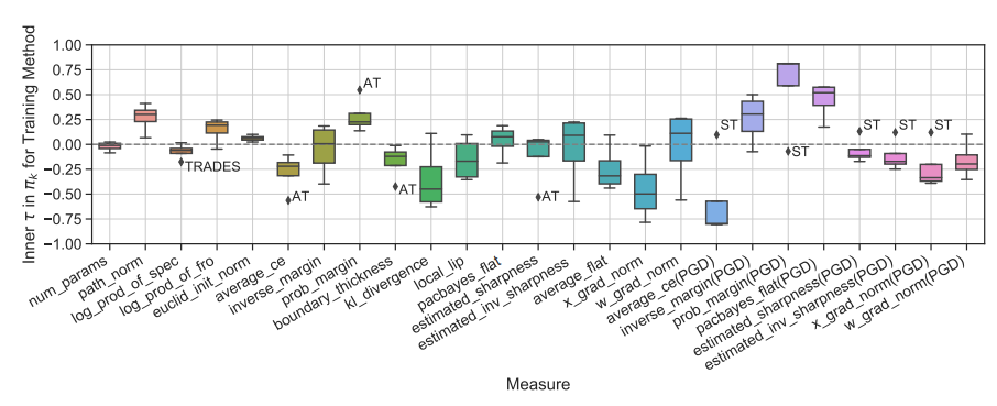
오히려, 기존에 강건성과 긴밀한 상관 관계가 있다고 알려진 마진(margin)이나 손실함수의 평평함(Flatness)는 기존 해석들과 정반대되는 모습을 보이기도 했습니다.

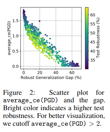
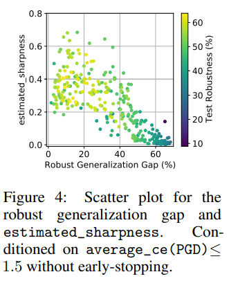
특정 조건 하에서는 기존에 주목을 잘 받지 못했던 입력 기울기의 크기(Input gradient norm)이 강건성 일반화 차이와 가장 높은 상관관계가 있음을 보이기도 했습니다.

본 논문은 자체적으로 학습한 1,300개 모델 이외에도, https://robustbench.github.io/에 업로드된 벤치마크(Benchmark) 모델에 대해서도 평가를 진행하였으며, 유사한 결과를 도출해내었습니다.

결론

강건성은 인공지능의 신뢰성 부문에서 핵심 개념 중 하나입니다. 모델의 강건성을 높이는 것은 미래 안전한 인공지능 사용을 위해 활발히 연구되어야 할 분야입니다. 본 연구는 ‘A 모델이 B 모델보다 이 특성이 좋아서 더 우수한 듯하다’라는 명제는 충분한 테스트 베드를 통해 검증되어야 함을 상기시키며, 보다 원활한 검증을 위해 PyTorch 기반의 적대적 방어 프레임워크 [MAIR]를 제안하였습니다. 다양한 특성에 대한 본 논문의 발견이 적대적 공격에 대한 강건성 분야의 발전에 기여하길 바랍니다.

관련 연구실 논문

• Understanding catastrophic overfitting in single-step adversarial training [AAAI 2021] | [Paper] | [Code]
• Graddiv: Adversarial robustness of randomized neural networks via gradient diversity regularization [IEEE Transactions on PAMI] | [Paper] | [Code]
• Generating transferable adversarial examples for speech classification [Pattern Recognition] | [Paper]