Introduction
When Artificial Intelligence (AI) models are deployed in real-world applications, it’s no longer sufficient for them to work most of the time. Instead, the more critical question is whether we can “trust these models”.
Adversarial Robustness refers to the concept of “Can a model function correctly even when an adversary manipulates specific noise into the input?” It is one of the biggest shortcomings that current AI is facing.
“Fantastic Robustness Measures: The Secrets of Robust Generalization” [Paper, Repo] is a paper presented by our lab at NeurIPS 2023. In this post, we first aim to explore the concept of adversarial robustness using basic mathematics and simple code examples.
Preliminary
Adversarial Examples and Adversarial Attacks
Source: https://adversarial-ml-tutorial.org/introduction/ [NeurIPS 2018 tutorial, “Adversarial Robustness: Theory and Practice”]
One of the best ways to understand adversarial robustness is by “creating adversarial examples.” Adversarial Examples are inputs where an attacker has inserted malicious noise into a benign input. This noise is often referred to as perturbation.
Let’s start by using a pre-trained ResNet50 model in PyTorch to classify a benign image of a pig.
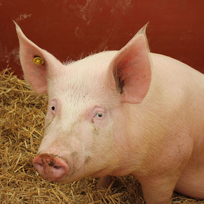
(1) First, read the image and resize it to 224x224.
from PIL import Image
from torchvision import transforms

# read the image, resize to 224 and convert to PyTorch Tensor
pig_img = Image.open("pig.jpg")
preprocess = transforms.Compose([
   transforms.Resize(224),
   transforms.ToTensor(),
])
pig_tensor = preprocess(pig_img)[None,:,:,:]

# plot image (note that numpy using HWC whereas Pytorch user CHW, so we need to convert)
plt.imshow(pig_tensor[0].numpy().transpose(1,2,0))
(2) After normalizing the resized image, load the pre-trained ResNet50 model to classify the image.
import torch
import torch.nn as nn
from torchvision.models import resnet50

# simple Module to normalize an image
class Normalize(nn.Module):
    def __init__(self, mean, std):
        super(Normalize, self).__init__()
        self.mean = torch.Tensor(mean)
        self.std = torch.Tensor(std)
    def forward(self, x):
        return (x - self.mean.type_as(x)[None,:,None,None]) / self.std.type_as(x)[None,:,None,None]

# values are standard normalization for ImageNet images,
# from https://github.com/pytorch/examples/blob/master/imagenet/main.py
norm = Normalize(mean=[0.485, 0.456, 0.406], std=[0.229, 0.224, 0.225])

# load pre-trained ResNet50, and put into evaluation mode (necessary to e.g. turn off batchnorm)
model = resnet50(pretrained=True)
model.eval()

# interpret the prediction
pred = model(norm(pig_tensor))

import json
with open("imagenet_class_index.json") as f:
    imagenet_classes = {int(i):x[1] for i,x in json.load(f).items()}
print(imagenet_classes[pred.max(dim=1)[1].item()])
hog
The model correctly identifies the image as a pig (“hog”). This is because the model has effectively minimized the following loss function during training:
\begin{equation} \label{eq:min} \min_\theta \ell(h_\theta(x), y) \end{equation}
Here, \(h\) represents the model, and \(\theta\) refers to the parameters of the model that are being optimized. By minimizing the loss function \(\ell\), we encourage the model to predict \(h_\theta(x)\) to be close to the true label \(y\) for the given input \(x\).
Adversarial examples, however, are designed to “fool the model.” Therefore, adversarial examples aim to maximize the loss function that was minimized during training.
\begin{equation} \label{eq:max} \max_{\hat{x}} \ell(h_\theta(\hat{x}), y) \end{equation}
This equation seeks to find a new image \(\hat{x}\) that maximizes the loss function \(\ell(h_\theta(\hat{x}), y)\). The resulting image or example is known as an adversarial example.
Moreover, the goal of an adversary is to create an example that, while still appearing to humans as a pig, leads the model to believe it’s something else. The noise \(\delta\) added to create the adversarial example \(\hat{x}=x+\delta\) must be subtle enough to go unnoticed by humans.
\begin{equation} \label{eq:max2} \max_{\delta\in\Delta} \ell(h_\theta(x+\delta), y) \end{equation}
The caculated noise \(\delta\) is referred to as an adversarial perturbation or adversarial noise.
Here’s how to implement this in PyTorch:
import torch.optim as optim
epsilon = 2./255

delta = torch.zeros_like(pig_tensor, requires_grad=True)
opt = optim.SGD([delta], lr=1e-1)

for t in 30:
    pred = model(norm(pig_tensor + delta))   # Add perturbation and predict
    loss = -nn.CrossEntropyLoss()(pred, torch.LongTensor([341]))  # Calculate loss
    if t % 5 == 0:
        print(t, loss.item())

    opt.zero_grad()
    loss.backward()  # Maximize the loss (note that we are minimizing negative loss)
    opt.step()
    delta.data.clamp_(-epsilon, epsilon)  # Limit size

print("True class probability:", nn.Softmax(dim=1)(pred)[0,341].item())
0 -0.0038814544677734375
5 -0.00693511962890625
10 -0.015821456909179688
15 -0.08086681365966797
20 -12.229072570800781
25 -14.300384521484375
True class probability: 1.4027455108589493e-06
Although this image still looks like a pig to human eyes, the model now classifies it with 99% confidence as a wombat.
Predicted class:  wombat
Predicted probability: 0.9997960925102234
This concept can be extended to create adversarial examples that manipulate the model to output whatever label we desire.
delta = torch.zeros_like(pig_tensor, requires_grad=True)
opt = optim.SGD([delta], lr=5e-3)

for t in range(100):
    pred = model(norm(pig_tensor + delta))
    loss = (-nn.CrossEntropyLoss()(pred, torch.LongTensor([341])) +
            nn.CrossEntropyLoss()(pred, torch.LongTensor([404])))
    if t % 10 == 0:
        print(t, loss.item())

    opt.zero_grad()
    loss.backward()
    opt.step()
    delta.data.clamp_(-epsilon, epsilon)
0 24.00604820251465
10 -0.1628284454345703
20 -8.026773452758789
30 -15.677117347717285
40 -20.60370635986328
50 -24.99606704711914
60 -31.009849548339844
70 -34.80946350097656
80 -37.928680419921875
90 -40.32395553588867
max_class = pred.max(dim=1)[1].item()
print("Predicted class: ", imagenet_classes[max_class])
print("Predicted probability:", nn.Softmax(dim=1)(pred)[0,max_class].item())
Predicted class:  airliner
Predicted probability: 0.9679961204528809
There are also many other adversarial attack methods to generate adversarial examples. For more information, refer to torchattacks.
Adversarial Robustness and Adversarial Defense
Since the discovery of adversarial examples in 2003, extensive prior work have tried to make models produce accurate predictions even in the presence of adversarial examples. Adversarial Robustness refers to the degree to which a model can withstand adversarial attacks. The methods aimed at improving robustness are known as Adversarial Defense techniques.
While many defense mechanisms have been proposed, one of the most actively researched is Adversarial Training (AT). Adversarial training teaches the model to correctly classify adversarial examples during training, much like how a vaccine works.
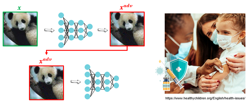
Mathematically, this becomes the following min-max problem:
\begin{equation} \min_{\theta} \max_{\hat{x}} \ell(h_\theta(\hat{x}), y) \end{equation}
To solve this min-max problem, various adversarial defense techniques (AT, TRADES, MART, etc.) have been proposed, leading to significant improvements in robustness. For more recent benchmarks, refer to https://robustbench.github.io/.
Main Results
Many different adversarial defense methods have been proposed to achieve high levels of robustness. In the process, some prior studies have aruged that “if a model possesses certain characteristics, then its robustness will improve.” Characteristics such as margin, boundary thickness, and Lipschitz constant have been frequently mentioned.
This paper examines whether these research hypotheses can be experimentally validated. A total of over 1,300 models were trained on the CIFAR-10 dataset under 8 different training environments (e.g., model architecture, adversarial defense techniques, batch size), and the characteristics of each model were measured to determine if they were meaningfully related to robustness.
Instead of focusing on the robustness itself, this paper measures the “Robust Generalization Gap,” which indicates how small the difference between robustness on the training set and the test set is. (※ The appendix provides evidence that simply measuring robustness does not yield meaningful results.)
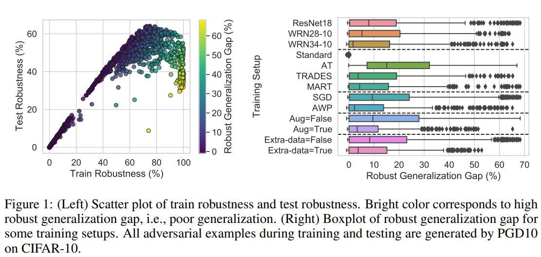
This paper reveal that none of the previously proposed characteristics are perfectly correlated with robustness. In particular, many characteristics show large variations depending on the adversarial defense technique used, with boundary thickness being a prominent example.
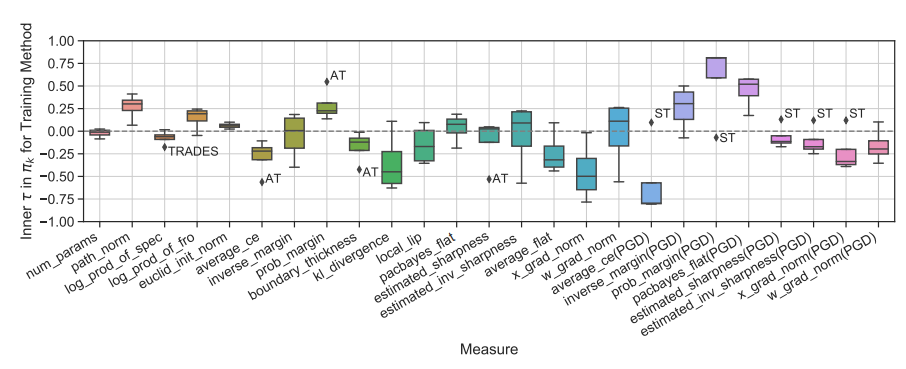
Contrary to previous observations, margin and loss function flatness, which were previously considered closely related to robustness, sometimes exhibited opposite behaviors.
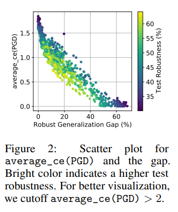
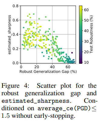
Under certain conditions, a characteristic that had not received much attention in prior work—input gradient norm—showed the highest correlation with the Robust Generalization Gap.

In addition to the 1,300 models trained by the authors, similar evaluations were conducted on benchmark models uploaded to https://robustbench.github.io/ yielding similar results.
Conclusion
Robustness is one of the core concepts in AI trustworthy. Improving model robustness is a critical area of research for the future safe use of AI. This study emphasizes that the hypothesis that “Model A is superior to Model B due to a certain characteristic” must be thoroughly validated through extensive testing environments. For more efficient validation, we propose the PyTorch-based adversarial defense framework [MAIR]. We hope the findings from this paper contribute to advancing the field of adversarial robustness.
Related Papers from the Lab
- Understanding catastrophic overfitting in single-step adversarial training [AAAI 2021] | [Paper] | [Code]
- Graddiv: Adversarial robustness of randomized neural networks via gradient diversity regularization [IEEE Transactions on PAMI] | [Paper] | [Code]
- Generating transferable adversarial examples for speech classification [Pattern Recognition] | [Paper]