Introduction
When Artificial Intelligence (AI) models are deployed in real-world applications, it’s no longer sufficient for them to work most of the time. Instead, the more critical question is whether we can “trust these models”.
Generalization refers to “Can the AI model perform well on examples it hasn’t seen during training?” It is a key element in ensuring the stable performance of AI.
“Stability Analysis of Sharpness-Aware Minimization” [Paper] is a paper from our lab that analyzes Sharpness-Aware Minimization (SAM), an optimization technique that enhances generalization performance. This article will explore both the concept of generalization and the paper.
Preliminary
Generalization and Generalization Gap
To understand generalization, one must first grasp the gap between the ideal and the reality that AI aims to achieve. Given a loss function \(\ell(\cdot)\) and parameters \(w\), an AI model aims to minimize the following:
\begin{equation} \min_w \mathcal{L}(w; \mathcal{S}) := \frac{1}{n} \sum_{(x, y) \in \mathcal{S}}\ell(w; x, y), \label{eq:erm} \end{equation}
where \(\mathcal{S}=\{x_i, y_i\}_{i=1}^n\) represents the accessible training dataset. This optimization method is known as Empirical Risk Minimization (ERM) and generally yields a good model under the statistical i.i.d. assumption.
However, in reality, the i.i.d. assumption is often violated, and due to limitations in the training data, we fail to achieve the ideal objective of “minimizing the loss function for all possible data” (equation below).
\begin{equation} \min_w \mathcal{L}(w; \mathcal{D}) := \mathbb{E}_{(x, y) \sim \mathcal{D}} \left[ \ell(w; x, y) \right]. \label{eq:erm_true} \end{equation}
Here, \(\mathcal{D}\) represents the true distribution of real data, including the unseen test data.
Thus, a gap arises between what the model learns \eqref{eq:erm} and what it aims to achieve \eqref{eq:erm_true}. This difference is defined as Generalization Gap \(\mathcal{E}(w)\).
\begin{equation} \mathcal{E}(w) = \mathcal{L}(w; \mathcal{S}) - \mathcal{L}(w; \mathcal{D}). \label{eq:truedistribution} \end{equation}
The smaller the \(\mathcal{E}(w)\), the smaller the performance difference between the training and real environments. Conversely, the larger the \(\mathcal{E}(w)\), the greater the gap between the two.
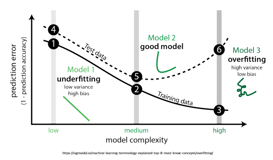
It is commonly said that a model is overfitted when the Generalization Gap \(\mathcal{E}(w)\) is significantly larger than expected, meaning the model performs well only on the training data.
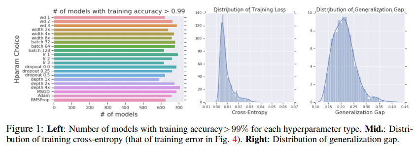
Prior research has shown that even if models trained under certain conditions achieve over 99% accuracy, the generalization gap can range from 0% to as high as 45%.
Sharpness-Aware-Minimization
Prior studies have proposed various methods to reduce the generalization gap \(\mathcal{E}(w)\), with a recent focus on the flatness of the loss landscape. The claim is that a model with a flat loss function in the parameter space (weight-space) will generalize better.
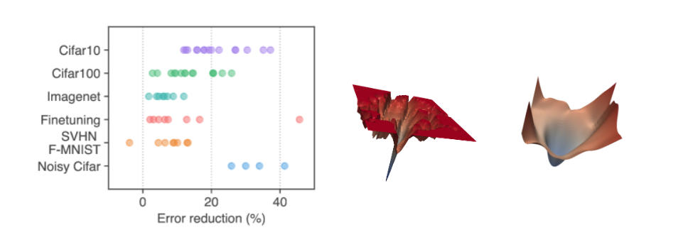
As seen in the image above, prior researchers demonstrated that a model with a flat loss function (right image) reduced errors much more effectively than one with a sharp loss function (middle image), as shown in the left image.
The Sharpness-Aware Minimization (SAM) optimization method was proposed to achieve such a flat loss function. Gradient Descent, a common optimization method, can be expressed as:
\begin{equation} w_{t+1} = w_t - \eta \nabla \ell(w_t), \label{eq:vanila} \end{equation}
where \(\eta\) is the learning rate, and \(\nabla\) is the gradient function.
The key idea of SAM is not only to reduce the current loss value but also to reduce the loss of the model with the highest loss within a neighborhood to make the loss function flatter.
\begin{equation} w^p_t = w_t + \rho \nabla \ell(w_t). \label{eq:wp} \end{equation} \begin{equation} w_{t+1} = w_t - \eta \nabla \ell(w^p_t), \end{equation}
This is formalized as shown above, where \(w^p\) represents the model with the highest loss value within a neighborhood \(\rho\).
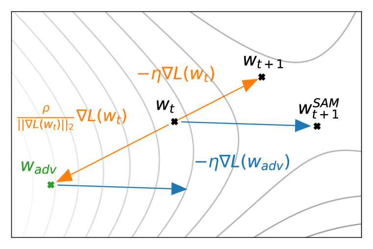

SAM has been used by various companies and researchers to improve model performance, and it was even used to train OpenAI’s generative model “Dall-e-2” by improving Clip.
Main Results
This paper begins with the question, “Does SAM always lead to better results?” The first experiment that sparked this paper is shown in the image below.
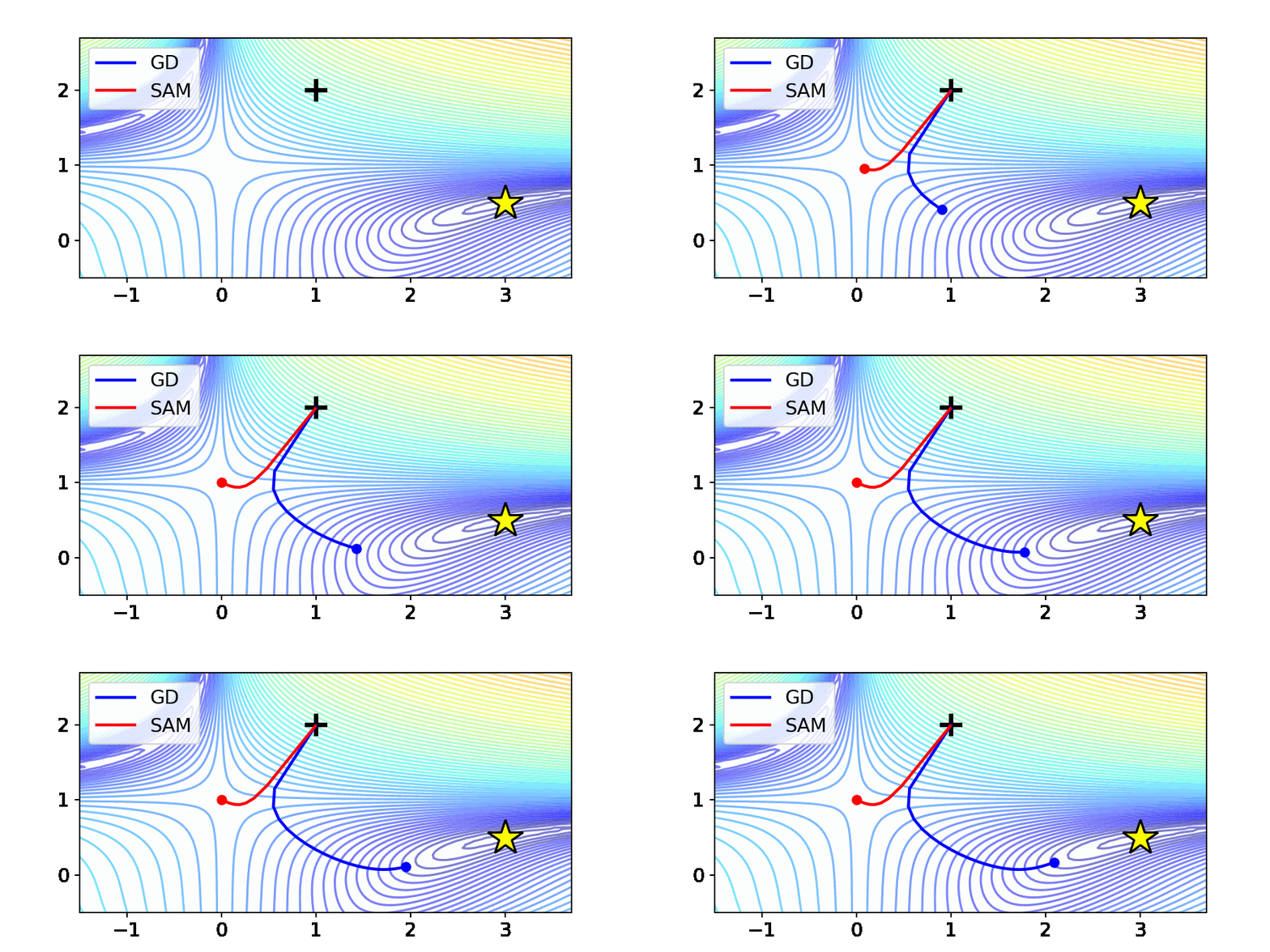
The image above shows the optimization results of Gradient Descent (GD) and SAM on the Beale function, commonly used in optimization. The Beale function has a saddle point at the center, and its minimum value is marked by a yellow star.
In the case of GD, it converges to the desired minimum point, the yellow star. In contrast, SAM fails to reach the optimal point and gets stuck at the saddle point. This paper refers to this phenomenon as the “Saddle point problem of SAM” and investigates SAM’s behavior theoretically and experimentally.
Saddle Point Becomes Attractor
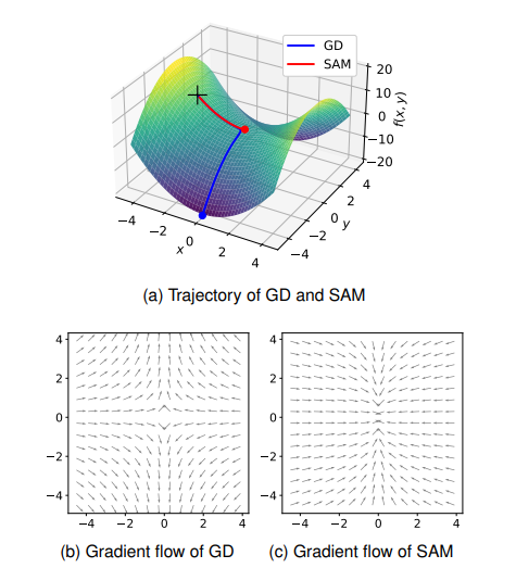
To further investigate SAM’s behavior, this paper analyzes the gradient flow using the simple function \(f(x, y) = x^2 - y^2\). The results reveal that while GD has gradient flows that allow it to escape from the saddle point, SAM exhibits a phenomenon where the saddle point becomes an attractor. In other words, although a saddle point typically cannot act as a point of convergence, under the SAM method, it behaves like one.

Stochastic Differential Equations on SAM
A typical Stochastic Differential Equation (SDE) can be expressed as follows:
\begin{equation} d w = -\nabla \ell(w^p) dt + [\eta C(w^p)]^{\frac{1}{2}} dW_t, \label{eq:dynamics} \end{equation}
By applying the SAM method to the stochastic differential equation above, the following proof is obtained:
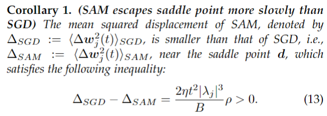
This behavior was also observed in experiments with deep learning models and batch-based learning.
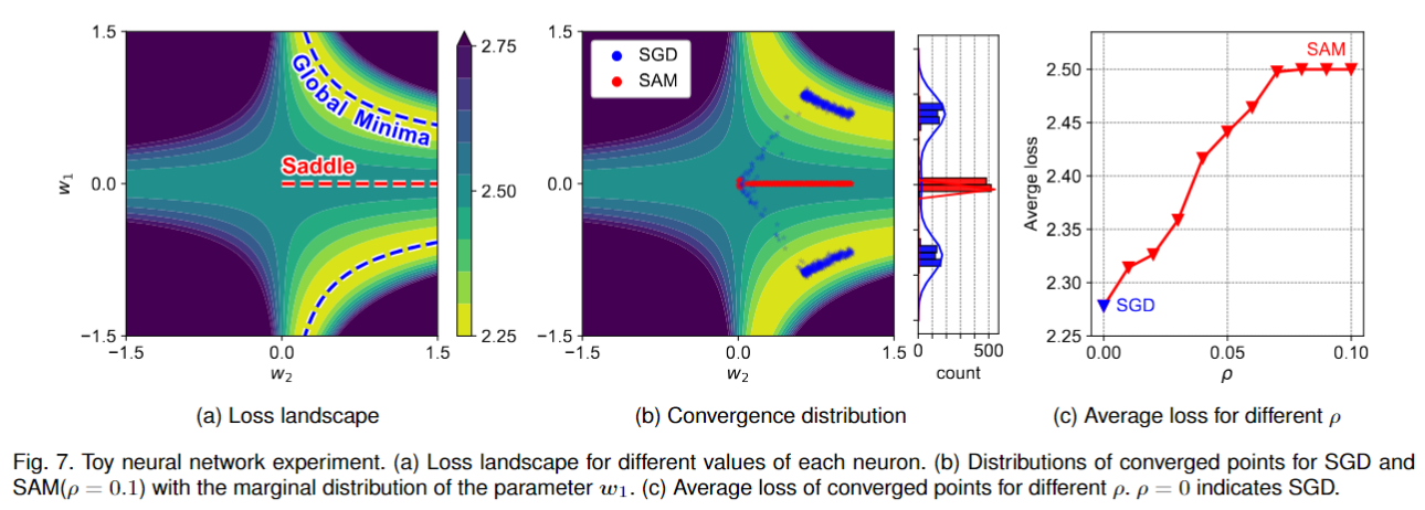
Thus, the paper demonstrates that SAM exhibits the saddle point problem not only when using full-batch gradient descent (GD) but also in batch-based learning compared to stochastic gradient descent (SGD).
Instability of Convergence and Training Techniques
So, how can we overcome the saddle point problem? This paper offers guidelines on adjusting training techniques to address this issue.
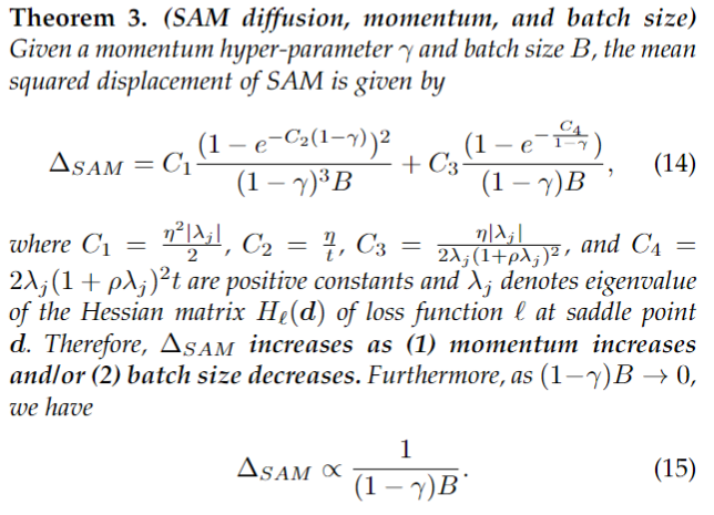
This proof suggests that increasing the momentum used in SAM or reducing the batch size increases the likelihood of escaping from the saddle point. Towards the end of the paper, this paper experimentally show that adjusting these training techniques is indeed effective in overcoming the saddle point problem.
Conclusion
Generalization is one of the key concepts in the reliability of AI. Enhancing the generalization performance of models means that the model performs similarly well in both limited environments and real-world environments. The field of generalization still has many mathematical and experimental challenges to be explored. This paper contributes to this effort by discussing the convergence problem of SAM through an analysis of its dynamics. We hope that the findings of this paper will contribute to the proposal of optimization methods that significantly improve the generalization performance of AI.
Related Papers from the Lab
- Differentially Private Sharpness-Aware Training [ICML 2023] | [Paper] | [Code]
- Fast sharpness-aware training for periodic time series classification and forecasting [Applied Soft Computing] | [Paper]
- Compact class-conditional domain invariant learning for multi-class domain adaptation [Pattern Recognition] | [Paper]