📖LLaVA Series: LLaVA-1, LLaVA-1.5

Paper: Visual Instruction Tuning

Authors: Haotian Liu, Chunyuan Li, Qingyang Wu, Yong Jae Lee

Venue: NeurIPS 2023

URL: https://arxiv.org/abs/2304.08485

---

Paper: Improved Baselines with Visual Instruction Tuning

Authors: Haotian Liu, Chunyuan Li, Yuheng Li, Yong Jae Lee

Venue: CVPR 2024

URL: https://arxiv.org/abs/2310.03744

LLaVA-1

---

Introduction

Earlier pretrained vision-language models were capable of performing a variety of visual tasks such as image classification, object detection, and image captioning. However, they had limitations when it came to serving as general-purpose assistants that could understand a user’s free-form questions and instructions and respond in a conversational manner.

Conversely, instruction-tuned LLMs could understand and carry out a wide range of natural language requests from users, but they could not directly process visual information such as images.

To bridge this gap, prior multimodal research added separate modules. For example, BLIP-2 used a trainable Q-Former between a frozen vision encoder and an LLM, while Flamingo inserted gated cross-attention layers inside the language model.

LLaVA explored whether a vision model and a language model could be effectively connected without such complex structures. To this end, it used CLIP ViT-L/14 as the visual encoder and Vicuna as the language model, placing only a single linear projection layer between the two models.

Therefore, the core of LLaVA lies not in designing a new, complex architecture but in converting existing image-text data into an instruction-following format and using it to endow the language model with the ability to carry out visual instructions.

Model Architecture

LLaVA consists of the following three components (see the figure below).

• Vision Encoder: CLIP ViT-L/14
• Connector: Linear projection layer
• Language Model: Vicuna-13B

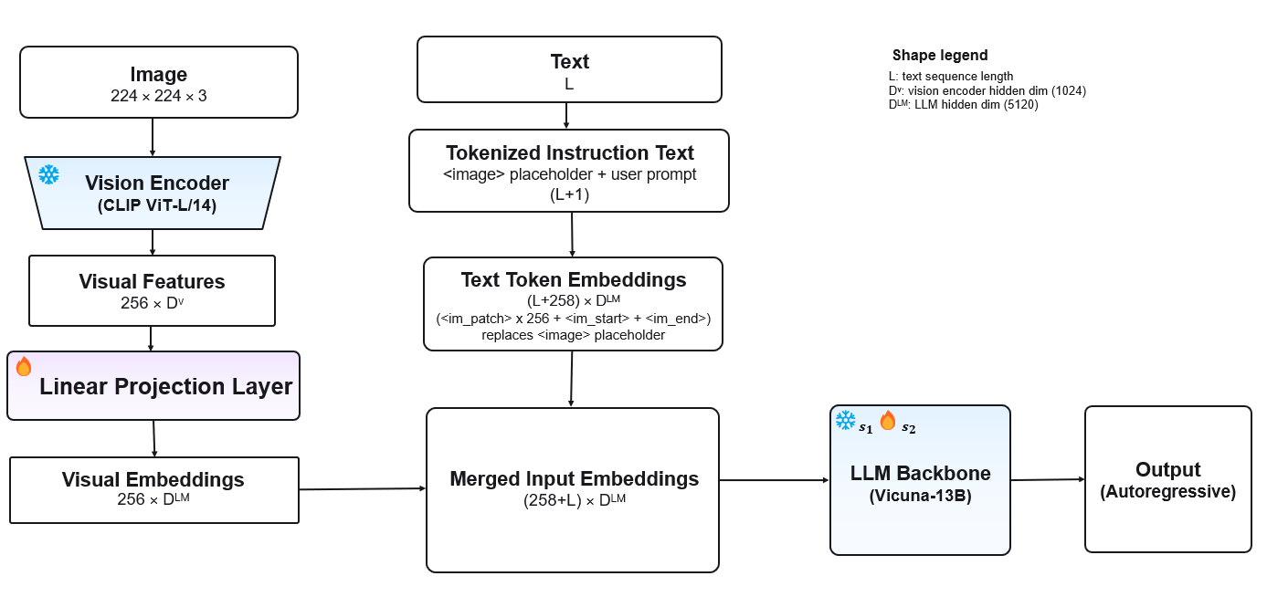
The input image $X_v$ is first resized to 224x224 and fed into CLIP ViT-L/14. CLIP then splits the image into 14x14 patches, so the entire image is converted into 256 patches (16x16). Each patch becomes a single visual token and is represented as 1024-dim.

The visual tokens then pass through the linear projection layer, where the feature size of each visual token is converted from 1024-dim to 5120-dim. This step aligns the visual features produced by CLIP with the text embedding space used by Vicuna. Even after the conversion, the number of visual tokens remains 256, but the feature size of each token becomes 5120-dim.

The text input $X_t$ is split into $N$ text tokens by the tokenizer, and each text token is converted into a 5120-dim vector as it passes through Vicuna’s embedding space.

The paper does not specifically state how the visual embeddings and text embeddings, produced through different paths, are combined into a single sequence; it only describes that the visual embeddings are inserted at the corresponding positions in the text sequence. The implementation in the official GitHub code is as follows.

LLaVA 1.0 code implementation (https://github.com/LLaVA-Annonymous/LLaVA)

The original prompt contains an <image> placeholder indicating where the image should be inserted. During preprocessing, a single <image> is converted into a form where <im_start>, <im_patch> repeated 256 times, and <im_end> are placed in order.

\[\langle\texttt{image}\rangle \longrightarrow \langle\texttt{im\_start}\rangle \underbrace{ \langle\texttt{im\_patch}\rangle \cdots \langle\texttt{im\_patch}\rangle }_{256\text{ tokens}} \langle\texttt{im\_end}\rangle\]

Here, the 256 <im_patch> tokens are not distinct tokens but the same special token repeated 256 times. Afterward, as the entire input passes through the tokenizer and Vicuna’s embedding layer, a 5120-dim token embedding is first generated at each position of <im_start>, <im_patch>, and <im_end> as well.

However, in the forward pass, the 256 <im_patch> embeddings are not used as they are. The model locates the 256 consecutive <im_patch> positions between <im_start> and <im_end>, and then replaces all of those embeddings with the 256 visual embeddings that have passed through the linear projection layer.

At this point, the embeddings of <im_start> and <im_end> are not replaced and are kept as they are. Therefore, the final input is constructed by concatenating, in order, the text embeddings before the image, the <im_start> embedding, the 256 visual embeddings, the <im_end> embedding, and the text embeddings after the image.

Thus, if the number of ordinary text tokens excluding the image-related special tokens is $N$, the final input consists of $N$+258 token positions, and each token has a 5120-dim feature.

Therefore, if there are $N$ text tokens, the combined input consists of $N$+256 tokens (or $N$+258 tokens in the paper’s code implementation), and each token has a 5120-dim feature. This combined multimodal sequence is fed into Vicuna, which processes the text and image information together and autoregressively generates the next text token based on the overall context.

Training Method

Autoregressive Training

For a single image $X_V$, LLaVA constructs multi-turn conversation data as follows: $(X_q^1, X_a^1, … , X_q^T,X_a^T)$, where $T$ is the total number of conversation turns, and $X_q^t$ and $X_a^t$ denote the $t$-th question and answer, respectively.

Note that the image is inserted only in the first turn, placed randomly either before or after the first question.

\[\mathbf{X}_{\mathrm{instruct}}^{t} = \begin{cases} \text{Randomly choose } [\mathbf{X}_{\mathrm{q}}^{1},\mathbf{X}_{\mathrm{v}}] \text{ or } [\mathbf{X}_{\mathrm{v}},\mathbf{X}_{\mathrm{q}}^{1}], & t=1,\\[3pt] \mathbf{X}_{\mathrm{q}}^{t}, & t>1. \end{cases}\]

Even though the image appears only once in the first turn, all subsequent questions are still part of the conversation about the same image, and the image tokens remain in the preceding context.

LLaVA uses Vicuna’s original next-token prediction objective as is. Letting the total number of target answer tokens be $L$, the conditional probability of the correct response is as follows.

\[p(\mathbf{X}_{\mathrm{a}} \mid \mathbf{X}_{\mathrm{v}}, \mathbf{X}_{\mathrm{instruct}}) = \prod_{i=1}^{L} p_{\boldsymbol{\theta}} \left( \boldsymbol{x}_{i} \mid \mathbf{X}_{\mathrm{v}}, \mathbf{X}_{\mathrm{instruct},<i}, \mathbf{X}_{\mathrm{a},<i} \right)\]

Here, $x_i$ is the assistant token to be predicted at the current step, $L$ is the number of target tokens, and $\theta$ denotes the parameters being trained at the current stage.

The important point is that no loss is computed on the user’s questions or the system message. The model receives these as conditioning input and is trained to predict only the assistant’s answer and the <STOP> token that marks the end of the conversation.

Stage 1 Training

Rather than training the entire model at once, LLaVA trains in two stages.

In the first stage, both CLIP and Vicuna are frozen, and only the projection layer connecting the two models is trained.

Training used approximately 595K image-caption pairs filtered from CC3M. The model is trained to take an image as input and generate the corresponding caption.

The purpose of this stage is not to learn new visual concepts from scratch. Since we already have CLIP, which represents visual information well, and Vicuna, which generates language well, only the way to connect the two models’ representation spaces is learned.

The paper describes this as the process of training a compatible visual tokenizer for the frozen LLM. That is, the projection layer converts CLIP features into a kind of visual token that Vicuna can understand.

Stage 2 Training

In the second stage, CLIP remains frozen, but not only the projection layer but also Vicuna is fine-tuned together.

Training used approximately 158K visual instruction data generated by GPT-4, as mentioned above. In this stage, the model learns not only to generate captions but also to answer questions appropriately, describe scenes in detail, and reason based on visual information.

Both stages use the same autoregressive objective. The difference lies in which parameters are trained and which data are used. If Stage 1 is the process of aligning the representation spaces of the two models, Stage 2 can be thought of as the process of learning the actual behavior of an assistant on top of that connection.

Dataset Generation

GPT-based instruction-response data generation

There are many large-scale datasets on the internet composed of images and captions. However, most of these data contain only Image+Caption correspondences.

This format is useful for learning the ability to briefly describe the content of an image, but it does not directly teach the ability to grasp a user’s question intent, hold multi-turn conversations, or perform step-by-step reasoning from an image. To solve this problem, instruction-response data was generated based on Image+Caption data.

LLaVA first converted existing image-caption pairs into the following instruction-following format using an image $X_V$, a caption $X_C$, and a question $X_q$ requesting a description of the image.

\[\texttt{Human}: \mathbf{X}_{\mathrm{q}}\, \mathbf{X}_{\mathrm{v}} \texttt{<STOP>} \quad \texttt{Assistant}: \mathbf{X}_{\mathrm{c}} \texttt{<STOP>}.\]

This approach is cheap and simple because the existing caption can be used directly as the answer. In fact, CC3M data converted into this format is used in Stage 1 of LLaVA. However, it has the limitation that the form of the questions and answers is simple, making it difficult to include detailed descriptions or complex reasoning.

Meanwhile, to create more diverse visual instruction data, LLaVA used a language-only GPT-4 as the teacher model. Since GPT-4 could not directly take images as input at the time, it was provided with the following two pieces of information as text instead of the actual image.

• Captions describing the image from various perspectives
• Bounding-box descriptions indicating the types and locations of objects

Using this information as a symbolic representation of the image, GPT-4 was made to understand the scene indirectly. Then, providing a few hand-crafted examples as in-context examples, three types of instruction-response data were generated (Conversation, Detailed Description, Complex Reasoning).

Data Type	Count	Main Purpose
Conversation	approx. 58K	Learns multi-turn conversations about objects, locations, actions, etc.
Detailed Description	approx. 23K	Learns the ability to describe a scene at length and in detail.
Complex Reasoning	approx. 77K	Learns the ability to reason about a situation based on visual cues.
Total	approx. 158K	Learns general-purpose visual instruction-following ability.

An important point in this process is that GPT-4 did not merely create questions. Based on the given captions and bounding boxes, GPT-4 generated both the questions and the answers. Therefore, instead of increasing the complexity of the architecture, LLaVA chose a data-centric approach of improving the format and quality of the training data.

Experimental Setup and Evaluation Method

Experimental Setup

• All models were trained on $8$ x A100 (NVIDIA GPU).

• Stage 1 fine-tuning settings
  • Epoch: $1$
  • Learning Rate: $2e^{-3}$
  • Batch Size: $128$
• Stage 2 fine-tuning settings
  • Epoch: $3$
  • Learning Rate: $2e^{-5}$
  • Batch Size: $32$

Evaluation Method

To measure the quality of the generated responses, the paper conducted a quantitative evaluation using GPT-4.

First, a pair of a text description and a question was constructed for each image. LLaVA then generated an answer based on the image and the question, while text-only GPT-4 took the text description and the question instead of the image and generated a reference answer serving as the comparison baseline.

After obtaining both models’ answers, the question, the visual information in text form, and the responses generated by GPT-4 and LLaVA were fed back into GPT-4. Here, GPT-4 acted as a judge evaluating the quality of the two responses.

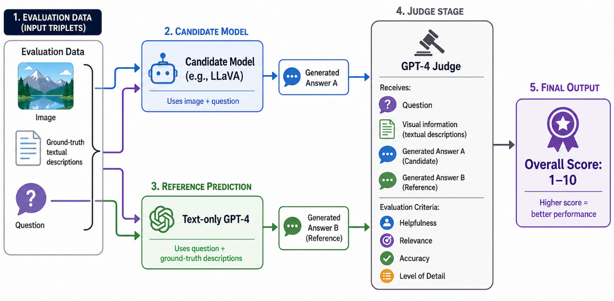
Each response was evaluated with an overall score from 1 to 10, where a higher score means better overall performance.

Note that the scores presented in the paper’s benchmark tables that follow are not a simple conversion of the 1-10 scores given by GPT-4, but relative scores computed by setting the total score of the GPT-4 reference response to 100.

\[\text{Relative Score} = 100\times \frac{\text{LLaVA response score}}{\text{GPT-4 reference score}}\]

Thus, for example, a score of 90 does not mean 90% accuracy but rather the relative response quality obtained compared to the GPT-4 reference in that evaluation.

Experimental Results

LLaVA-Bench(COCO)

LLaVA-Bench COCO consists of 30 images randomly selected from COCO-Val-2014. For each image, one Conversation, Detailed Description, and Complex Reasoning question was generated, for a total of 90 questions.

The model without instruction tuning scored only an average of 21.5. In contrast, the model using all three types of instruction data obtained 85.1.

This result shows that image-caption pretraining alone makes it difficult to follow a user’s various instructions. Furthermore, performance was higher when multiple types of data such as Detailed Description and Complex Reasoning were used together in training than when only Conversation data was used. Instruction data of different formats also had a positive effect on the model’s general conversational ability.

LLaVA-Bench(In-the-Wild)

The In-the-Wild benchmark consists of 24 images and 60 questions. It includes not only ordinary photos but also various domains such as memes, sketches, paintings, and indoor and outdoor scenes.

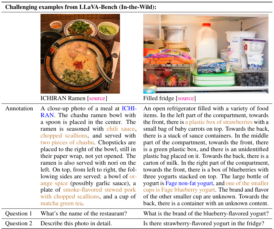
LLaVA obtained an overall score of 67.3, outperforming BLIP-2 and OpenFlamingo. In particular, it recorded 81.7 in Complex Reasoning, showing a large margin.

This shows that LLaVA has a strength in grasping the user’s question intent and reasoning about visual information accordingly.

ScienceQA

ScienceQA is a benchmark consisting of approximately 21K school-level multiple-choice questions. It covers various subjects such as natural science, social science, and language science, and depending on the question, text or images are provided alongside it.

The LLaVA for ScienceQA did not use the general chatbot model as is, but was separately fine-tuned for 12 epochs to fit that dataset. The question and additional context were used as the instruction, and the reasoning and final answer were composed as the target response.

The main results are summarized in the table below.

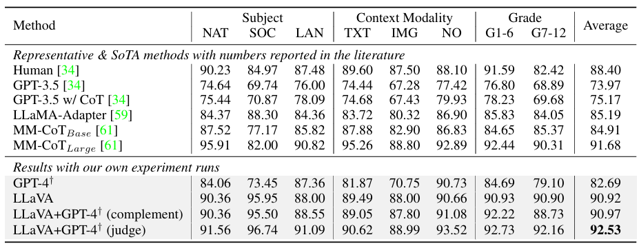
The LLaVA standalone model achieved 90.92% accuracy, approaching MM-CoT large, the top-tier model at the time.

GPT-4 complement used LLaVA’s answer for questions that GPT-4 could not answer, but its performance was 90.97%, almost no different from LLaVA alone.

On the other hand, GPT-4 (judge) had GPT-4 choose the final answer between the two candidates when LLaVA’s and GPT-4’s answers differed. This approach recorded 92.53%, achieving new SOTA performance at the time of the paper’s publication.

The GPT-4 (judge) in ScienceQA must be distinguished from the evaluation method of LLaVA-Bench. In LLaVA-Bench, a score is assigned to the quality of the response, whereas in ScienceQA it is used as an ensemble method that selects one final correct answer between two candidates.

The ScienceQA experiments also analyzed the effect of each design element on performance.

• When the 23rd layer feature of CLIP was used instead of the 24th layer, accuracy increased from 89.96% to 90.92%.
• When Stage 1 feature alignment was omitted, accuracy decreased to 85.81%.
• Generating reasoning before the answer did not make a large difference in final performance, but reached similar accuracy with fewer epochs.
• Vicuna-7B recorded 89.84%, and Vicuna-13B recorded 90.92%.

The most striking part of these results is the effect of Stage 1. When feature alignment was omitted, a performance drop of about 5.11% occurred. This shows that training the projection layer is an important process for learning visual-language alignment.

Conclusion

LLaVA 1.0 is a study that showed a general-purpose visual assistant can be built through visual instruction tuning.

The structure itself is very simple, consisting of CLIP, a linear projection layer, and Vicuna. However, by combining Conversation, Detailed Description, and Complex Reasoning data generated by GPT-4 with two-stage training, it learned the abilities of conversing about images, describing them in detail, and complex reasoning.

The effect of instruction tuning appeared in the experiments as well. It obtained 85.1 points on LLaVA-Bench COCO and 67.3 points on In-the-Wild, and on ScienceQA it recorded 90.92% on its own and 92.53% when combined with the GPT-4 judge.

The main contributions of this paper can be summarized in three points.

First, it presented a visual instruction tuning method that converts existing image-caption data into an instruction-following format. Second, it generated approximately 158K diverse visual instruction data using GPT-4. Third, by open-sourcing LLaVA-Bench, the model, and the training data, it laid the foundation for subsequent vision-language assistant research.

The core of this paper is that a complex architecture is not always necessary. If there are already well-trained vision encoders and language models, a powerful multimodal assistant can be built with just a simple projection layer connecting the two models and appropriate instruction data.

Of course, limitations also exist. LLaVA sometimes fails to accurately understand detailed visual information or relationships between objects, and it also has the hallucination problem of generating content that does not exist in the image. In addition, it relies heavily on GPT-4 in the data generation and evaluation processes, and LLaVA-Bench also has the limitation of being composed of a relatively small number of images and questions.

Therefore, the greatest significance of LLaVA lies not in the new model architecture itself, but in presenting GPT-based data generation, visual instruction tuning, a new benchmark, and open-source release as a single framework. This approach can be assessed as having laid an important foundation for the subsequent full-scale spread of large-scale vision-language model research.

LLaVA-1.5

---

Multimodal models such as LLaVA-1 and MiniGPT-4 introduced above demonstrated, through visual instruction tuning, the ability to answer images and questions in accordance with instructions and to reason about images. These models improved performance by scaling up pretraining data, instruction-following data, vision encoders, language models, and so on.

However, the optimal recipe for a general-purpose model had not been clearly established. For example, when comparing LLaVA-1 and InstructBLIP, LLaVA-1 was better at conversationally reasoning about images, while InstructBLIP was better on VQA benchmarks that require a single word or short-form answer as the correct answer.

This paper studies how to adjust the detailed settings and training methods, while minimizing changes to the LLaVA-1 model architecture, so as to build a model with the best general-purpose performance. And the resulting model built with that optimal method is LLaVA-1.5.

Unsolved Challenges of Existing Large Multimodal Models (LMMs)

Although LMMs showed good performance, several problems still remained to be solved.

The first is the process of handling high-resolution images. CLIP-ViT-L/14, the vision encoder frequently used by LMMs, can only take 224 x 224 pixel images as input, so larger-resolution images inevitably had to be turned into 224 x 224 form through methods such as resizing, cropping, and padding. However, in such cases, there was a risk of losing the detailed information contained in high resolution.

The second is the compositional capabilities of each task. Compositional capability is the ability to perform some new task that requires the ability to perform all of several different tasks, even when each task is trained separately. For example, suppose one LMM is trained on pairs of images and English text, and separately trained on multilingual text data. A model with compositional capability can interpret images in multiple languages even without explicitly learning image-multilingual pairs.

The third is data efficiency. The more data required for training, the more time it takes to train, so the key is how to boost the model’s performance with as little data as possible.

In this paper, the authors seek answers to these unsolved challenges through LLaVA-1.5.

Detailed Changes in LLaVA-1.5

Unlike the previous LMM models with their complex structures, the previous LLaVA-1 model showed performance similar to or better than earlier models with just a single linear projection layer.

However, LLaVA-1 was not perfect in every respect. Compared to the earlier model InstructBLIP, LLaVA-1 underperformed InstructBLIP on academic benchmarks that typically require short-form responses. Conversely, LLaVA outperformed InstructBLIP in the ability to handle real-world images and conversational tasks about them.

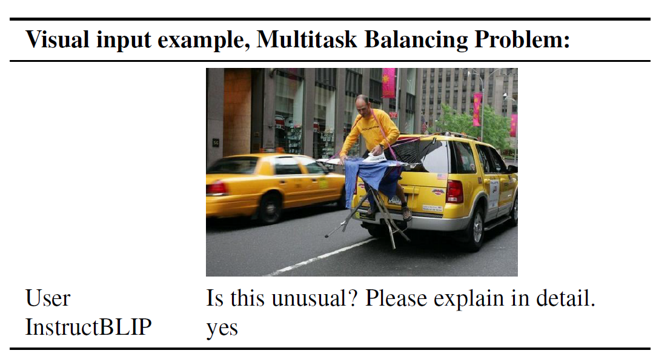
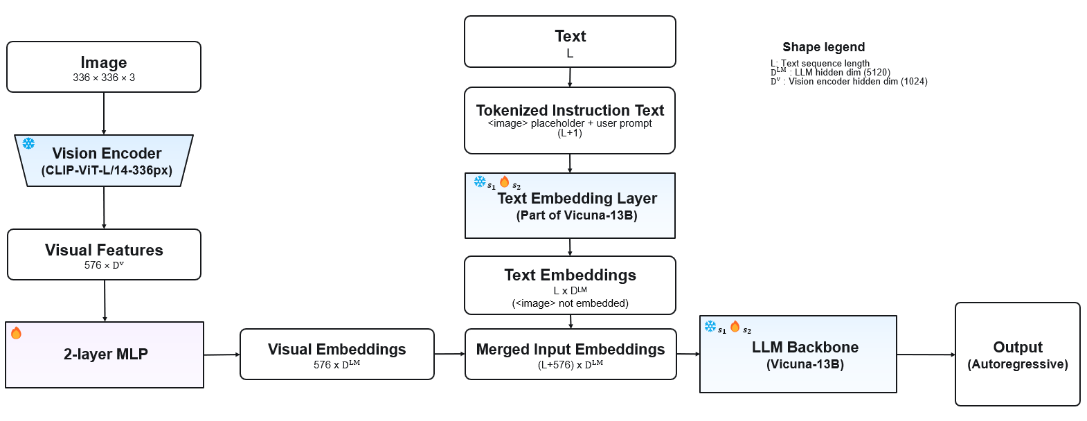
The authors succeeded in implementing LLaVA-1.5, a general-purpose model, while minimizing changes to the LLaVA-1 model. Other than changing the single linear projection layer of the original LLaVA-1 into a two-layer multi-layer perceptron (MLP), LLaVA-1.5 made no major changes to the model architecture. Simply by changing or adding fine-tuning datasets and scaling up the LLM or vision backbone, it achieved SOTA on various benchmarks.

Let us look specifically at what changes LLaVA-1.5 made.

Response Format Prompting

One of the problems of the existing models was that it was difficult to find a balance between long, sentence-form answers and short answers.

The authors judged that the reason was the ambiguity of the prompt. A prompt like Q : {Question} A : {Answer} is not sufficient to tell the model the desired form of the answer. To solve this, the authors added a short but clear prompt {“Answer the question using a single word or phrase”} after the VQA question.

They also pointed out that one reason such a problem occurred in InstructBLIP was that the LLM was kept frozen throughout the fine-tuning stage, and when training LLaVA-1.5, the LLM was fine-tuned as well.

Scaling the Data and Model

In addition to the Response Format Prompting described above, LLaVA-1.5 performed fine-tuning with more diverse data compared to LLaVA-1.

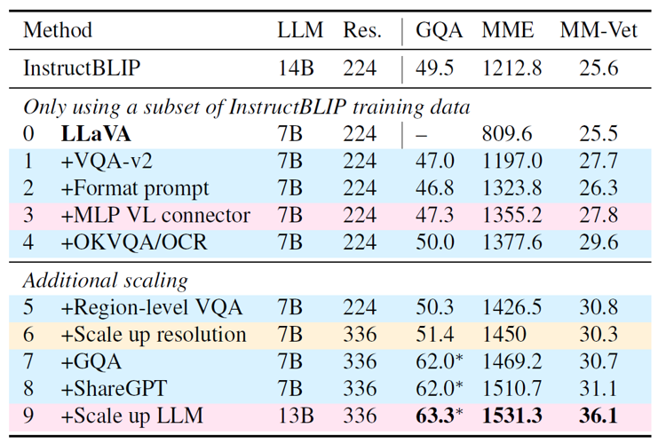
The paper started by taking the initial LLaVA-1 model and measured performance changes while sequentially stacking additions of fine-tuning data, model modifications, resolution modifications, and so on.

In the table above, the parts marked in blue represent data additions, red represents model architecture modifications, and yellow represents modifications to the input image resolution. The GQA, MME, and MM-Vet benchmarks are benchmarks that evaluate multimodal ability through short-answer questions, questions with an output format, and questions that ask the model to describe an image in prose, respectively. The 7B model reflected up to row 8 and the 13B model reflected up to row 9 are called LLaVA-1.5 (7B, 13B).

The resolution enhancement part marked as row 6 represents changing the vision encoder backbone from CLIP-ViT-L, which supports 224x224 image input, to CLIP-ViT-L-336px, which supports 336px.

Row 3, as mentioned earlier, is the change of the single linear projection layer to an MLP, and row 9 is the change of the existing LLM backbone from Vicuna-7B to Vicuna-13B.

LLaVA-1.5 used the same pretraining data as LLaVA-1 and achieved much better performance while keeping the iteration and batch size almost identical.

Scaling to Higher Resolutions

Although LLaVA-1.5 seemed to have solved the resolution problem by changing the vision encoder backbone to CLIP-ViT-L-336px, it still could only take images at 336x336 resolution, so the problem was not fundamentally solved. To address this, the authors proposed a method of splitting a high-resolution image into a grid and feeding each cell into the ViT encoder separately.

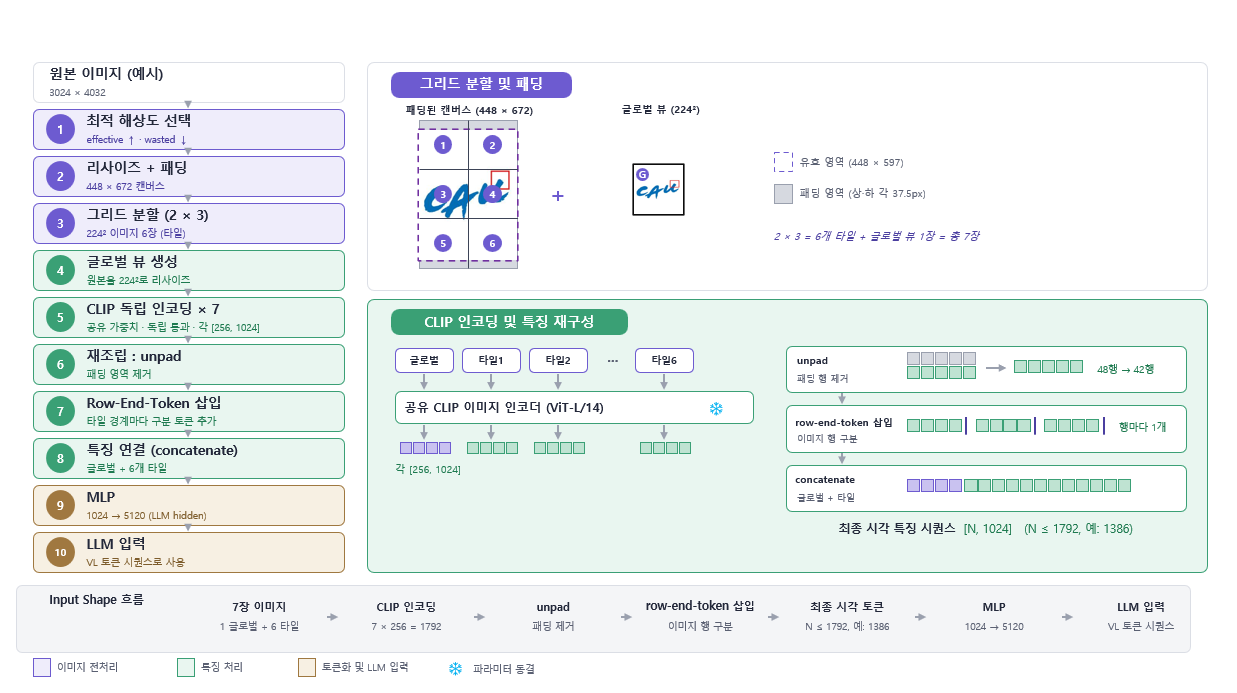
When using this method, the encoder backbone used CLIP-ViT-L, which takes 224x224 pixel images as input. That is, the size of one grid cell is 224x224.

First, an appropriate grid to process the image is predefined. The predefined grids include 1x1, 1x2, 1x3, 1x4, 1x5, 1x6, 2x2, 2x3 and their respective transposes. When a high-resolution image comes in, the grid that can best represent that image is selected. The criterion for selecting the grid is to choose the grid that represents the image’s detailed information as well as possible while minimizing wasted area. After that, the image is downscaled to fit that grid while maintaining the original aspect ratio. At this point, the ratio is adjusted so that the entire image fits within the grid without being cut off. The empty space created in the grid as the image is downscaled is filled with padding.

The problem with this process is that attention cannot be performed between the image pieces placed in each grid cell. Because each cell is fed into the vision encoder separately, the model cannot learn the relationships between the cells. To solve this, in addition to individually encoding the image piece in each cell, the entire image is downscaled to one grid-cell size, i.e., a global view is created, and encoding is additionally performed. This global view is finally concatenated to the flattened vector of each cell’s image encoding and computed.

Once each cell is encoded, the vector is reassembled to reflect the width and height of the original image. Then the padding areas are removed to prevent resource consumption. Also, since the reassembled vector is subsequently flattened, a row end token is added at the end of each row so that the model can know, even after flattening, that they were in the same row. After the vector is flattened, the global view vector is concatenated to complete the final vector.

This vector then passes through an MLP and is projected into the input space of the LLM backbone to be used as the LLM’s input.

The authors named the model using this method LLaVA-1.5-HD.

Experiments and Evaluation

Benchmark Performance

Performance evaluation was conducted with academic-task-oriented benchmarks (VQA-v2, GQA, VizWiz, etc.) and recently proposed LMM benchmarks for evaluating instruction-following ability (POPE, MME-Perception, MMBench, etc.). Each benchmark evaluates various abilities such as short-answer questions, multiple-choice questions, reasoning ability, and the degree of hallucination.

The results for each experiment are shown in the following table.

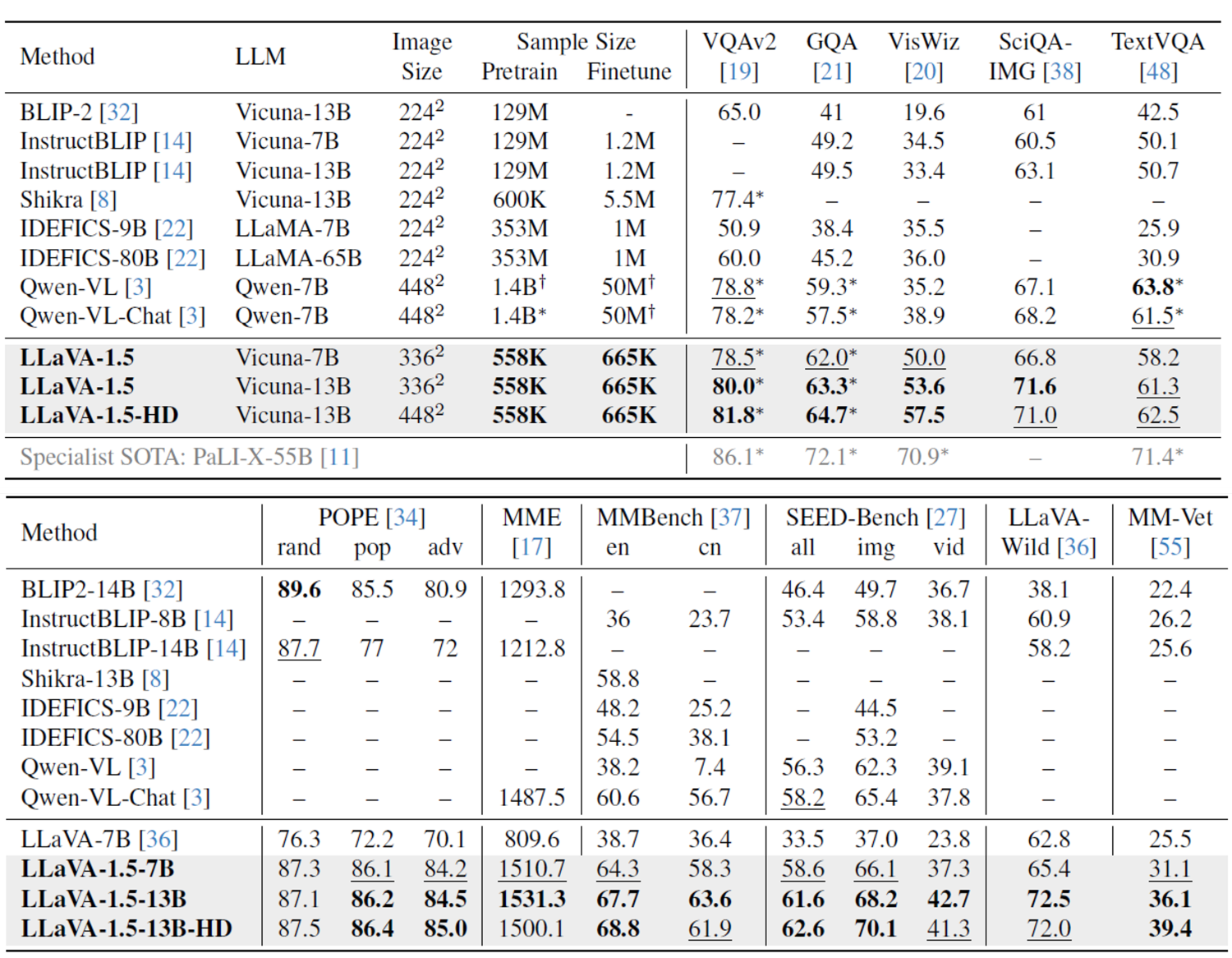
LLaVA-1.5 achieved SOTA in most areas, and showed better performance when using a 13B model than when using a 7B-parameter LLM backbone.

Also, when the LLaVA-1.5-HD model was made able to process images in 448x448 form, it showed performance improvements on most benchmarks, and showed especially larger improvements on benchmarks requiring more detailed understanding of images, such as MM-Vet’s OCR and the LLaVA-Bench-in-the-Wild benchmark.

Ablation

As an ablation, we experimented with how much the benchmark performance differs when the LLM backbone model is changed and when only 10-50% of the original amount of fine-tuning dataset is used.

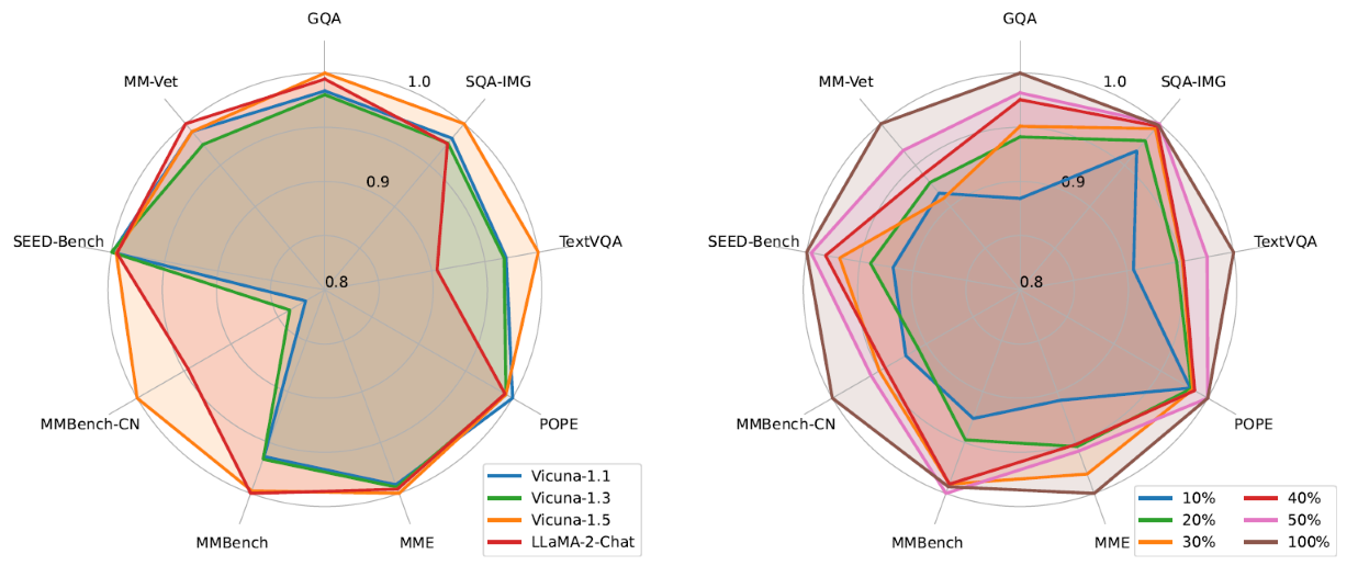
First, for the LLM backbone model, Vicuna-1.1 and 1.3 based on LLaMA-1, Vicuna-1.5 based on LLaMA-2, and LLaMA-2-Chat were used for comparison. The Vicuna series is a model fine-tuned only with supervised instruction fine-tuning (SFT), while LLaMA-2-Chat is a model additionally trained with reinforcement learning from human feedback (RLHF).

Looking at the benchmark experiment results, the model using Vicuna-1.5 performed best, and the models using LLaMA-2-based LLMs performed better than the models using LLaMA-1-based LLMs. Through this, it was confirmed that the performance of a VLM is greatly affected by the performance of the LLM.

One notable point is the performance of the models using Vicuna-1.5 and LLaMA-2-Chat on the MMBench and MMBench-CN benchmarks. On the English-language MMBench, the models using the two language models performed similarly, but on the Chinese-language MMBench-CN, Vicuna-1.5 showed markedly superior performance.

This is because, whereas the SFT/RLHF data used in training LLaMA-2-Chat was mostly English, Vicuna-1.5 was SFT’d on ShareGPT, which includes a large amount of multilingual data. Through this, we can see that what abilities the backbone LLM’s instruction tuning data contains determines the performance on benchmarks requiring those abilities.

Also, looking at the benchmark performance of the models that used only 10%-50% of the fine-tuning dataset by random sub-sampling, we can confirm that no large performance drop occurred up to 30-50%. On MMBench, the model using only 50% was even found to perform better than when using 100%. This can be interpreted as meaning that there is room left to further increase data efficiency.

Hallucination

The hallucination of existing LMMs had been thought to be caused by errors or hallucinations within the training dataset.

However, in this study, when the model’s input resolution was increased to something like 448x448, the hallucination phenomenon was confirmed to decrease markedly.

This means that even though the model’s input resolution is not high enough to represent the image’s detailed information, if the model is asked for fine-grained information beyond its capability, the model learns to hallucinate.

Conclusion

---

If LLaVA-1 proposed the hypothesis that “we compete on data quality with only a linear projection, without a complex connector,” LLaVA-1.5 systematically verified that recipe in a controlled setting.

The most noteworthy result is efficiency. LLaVA-1.5, with only 558K pretraining + 665K instruction tuning data, surpassed InstructBLIP (129M) and Qwen-VL (1.4B), which trained visual resamplers on hundreds of millions to billions of pairs, as well as the 80B-scale IDEFICS. Considering even that the entire training finishes within a day on 8×A100, it is, in the authors’ words, a result that makes one reconsider the very benefits of a visual sampler such as Q-Former and the necessity of large-scale vision-language pretraining.

LLaVA-1.5 also left interesting observations about the unsolved challenges of LMMs.

The points that more than 98% of performance is maintained even when using only 50% of the data (data efficiency), that hallucination is greatly reduced when resolution is increased (the need for a balance between data detail and model capacity), and that individual abilities are composed and generalize to new tasks even without explicit joint training (compositional capability).

However, it states that problems such as multi-image understanding and hallucination are still challenges to be solved.