Paper: Adversarial Examples Are Not Bugs, They Are Features
Authors: Andrew Ilyas, Shibani Santurkar, Dimitris Tsipras, Logan Engstrom, Brandon Tran, Aleksander Madry
Venue: NeurIPS 2019
Introduction
An adversarial example is an input that looks nearly identical to the original to a human observer, yet distorts a deep learning model’s prediction. Prior work has primarily attributed this phenomenon to model fragility, properties of high-dimensional input spaces, overfitting, insufficient training data, or anomalies near the decision boundary. In other words, adversarial examples have often been understood as a kind of bug caused by the model’s failure to learn properly.
This paper, however, argues that adversarial examples are not simply bugs but rather the consequence of features the model has actually learned. Within the training data there exist features that are nearly invisible to human eyes but useful for predicting the correct label, and the model learns these features in order to improve accuracy. Some of these features, however, can have their predictions easily flipped by small perturbations, and the paper explains that adversarial examples fool the model precisely because standard training exploits these features.
Definitions of Features
Terminology
| Term | Meaning |
|---|---|
| Feature | Information extracted from the input data |
| Useful feature | A feature correlated with the true label, helpful for classification |
| Robust feature | A feature whose relationship with the label is preserved even under small perturbations |
| Non-robust feature | A feature that is normally helpful for classification but is easily flipped by small perturbations |
| Standard training | Training that minimizes loss to maximize standard accuracy |
| Robust training | Training that accounts for the worst-case perturbation an attacker could add |
| Transferability | The phenomenon in which an adversarial example crafted for one model also fools another |
-
Adversarial example
An adversarial example is an input \(x + \delta\) formed by adding a small perturbation \(\delta\) to a clean input \(x\). The perturbation \(\delta\) is designed to be imperceptible to humans while either substantially increasing the model’s loss or steering its prediction toward a specific class.
A typical adversarial attack can therefore be expressed as follows.
\[x_{adv} = x + \delta\] -
Feature
The paper defines a feature as a function from the input space to the real numbers.
\[f: X \rightarrow \mathbb{R}\]That is, a feature is some measurement extracted from an image. It might be a familiar attribute such as “a dog’s ear,” or it might be a pixel-level statistical pattern that humans hardly perceive at all. Crucially, from the model’s perspective these are not fundamentally different: if a feature helps predict the correct label, the model will use it.
-
Useful feature
If a feature \(f\) is, on average, positively correlated with the label \(y\), the paper calls it a useful feature. In other words, if observing a feature helps predict the correct answer, it is a useful feature. In the equation below, \(\rho\) measures the degree to which the feature is associated with the label.
\[\mathbb{E}_{(x,y)\sim D}[y \cdot f(x)] \geq \rho\] -
Robust feature
A useful feature is robust if it continues to align with the label even when the attacker adds a small perturbation. In the equation below, \(\Delta(x)\) is the set of perturbations available to the attacker. That is, even when the attacker shifts the input in the worst possible direction, if the useful feature still helps predict the correct label, it is considered robust.
\[\mathbb{E}_{(x,y)\sim D} \left[ \inf_{\delta \in \Delta(x)} y \cdot f(x+\delta) \right] \geq \gamma\] -
Non-robust feature
Non-robust features are the central concept of this paper. They are features that are normally helpful for predicting the correct label (and therefore useful), but whose relationship with the label is easily broken or even reversed by a small perturbation.
For example, suppose a dog image contains a faint pattern that is barely visible to the human eye but is statistically tied to the dog label. A model that learns this pattern will see its accuracy improve. But if an attacker slightly modifies the pattern, the model may now classify the image as a cat. In this case, the pattern is a useful but non-robust feature.
Training Methods
-
Standard training
The goal of ordinary supervised learning is to reduce loss on the training data and improve accuracy on the test data. In this process, the model does not consider whether a feature is “natural” or “stable under attack.” What matters is whether the feature improves accuracy. The paper formalizes this as follows.
\[C(x) = \operatorname{sgn} \left( b + \sum_{f \in F} w_f \cdot f(x) \right)\]The classifier \(C\) predicts based on a weighted combination of various features. If a feature helps predict the label, the model uses its weight to reduce loss. Within this objective, no distinction is drawn between robust and non-robust features. In other words, standard training uses every feature that helps the model predict the correct label. As a result, non-robust features are also learned, because while they are vulnerable to attacks, they genuinely improve accuracy under normal conditions.
-
Robust training
Robust training also takes into account the situation where the attacker has distorted the input. Whereas ordinary training minimizes the loss on the original input \(x\), robust training considers the worst-case perturbation \(\delta\) within an allowed set that maximizes the loss.
\[\mathbb{E}_{(x,y)\sim D} \left[ \max_{\delta \in \Delta(x)} L_\theta(x+\delta, y) \right]\]Under this training scheme, relying on non-robust features is dangerous, since the attacker can flip them easily. Robust training can therefore be understood as a process that prevents the model from relying too heavily on combinations of useful but non-robust features.
This can be summarized as follows.
| Training Method | Tendency of What the Model Learns |
|---|---|
| Standard training | Uses every feature that helps accuracy |
| Robust training | Prefers features that are hard for the attacker to manipulate |
Separating Robust and Non-Robust Features
Objective
This experiment attempts to separate robust features from non-robust features. The goal is to verify whether a robust model can be obtained by performing standard training on robust features alone, instead of through adversarial training.
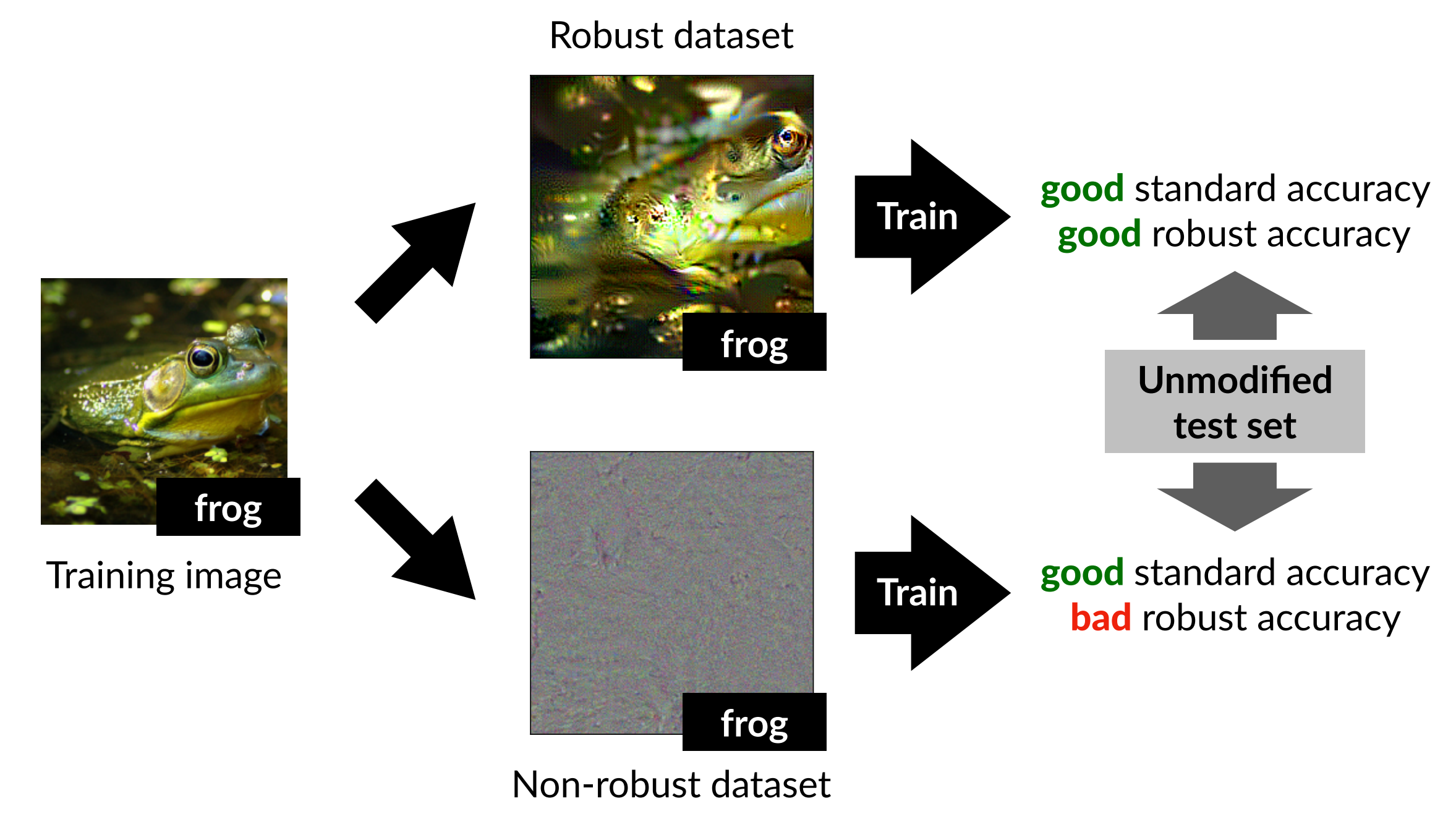
Robustified Dataset
First, we need to construct a robustified dataset by removing non-robust features from the training data \(D\). To do so, we use a robust model that has been pre-trained via adversarial training. The representation layer (just before the final linear classifier) of this robust model can be regarded as the set of features the robust model uses for classification. Therefore, if we craft a new image \(x_r\) such that its internal representation in the robust model is similar to that of the original image \(x\), the features used by the robust model are preserved in \(x_r\). This can be expressed as the following optimization problem.
\[\min_{x_r} \|g(x_r) - g(x)\|_2\]Here, \(g(x)\) denotes the result of passing the input \(x\) through the robust model up to its representation layer. \(x_r\) is then optimized via gradient descent. Importantly, the authors do not start the optimization from the original image. Instead, they begin from a different image (chosen independently of the label) or from random noise. The reason is to ensure that features the robust model does not use are not correlated with the original label.
The dataset constructed in this way serves as the robustified dataset \(\hat{D}_R\). Although the robustified dataset may not look entirely natural to a human, it is constructed so that, at the representation layer of the robust model, its activation values are similar to those of the original image.
\[\mathbb{E}_{(x,y)\sim \hat{D}_R}[f(x)\cdot y] = \begin{cases} \mathbb{E}_{(x,y)\sim D}[f(x)\cdot y], & f \in F_C \\ 0, & \text{otherwise} \end{cases}\]The equation above defines, for the newly constructed \(\hat{D}_R\), the degree of correlation between feature \(f\) and the true label \(y\). Here, \(F_C\) is the set of features used by the robust classifier \(C\). That is, the features actually used by the robust model retain the same predictive power as in the original dataset, while the remaining features are made uncorrelated with the label.
Non-Robust Dataset
The non-robust dataset \(\hat{D}_{NR}\) is constructed via the same optimization scheme, but using a standard model in place of a robust model. A standard model uses both robust and non-robust features, but because it has not undergone adversarial training, it is regarded as a model with low robustness that focuses on non-robust features.
Results
After separating \(D\) into \(\hat{D}_{R}\) and \(\hat{D}_{NR}\), the accuracy and robustness obtained when each is used as the training set are evaluated.
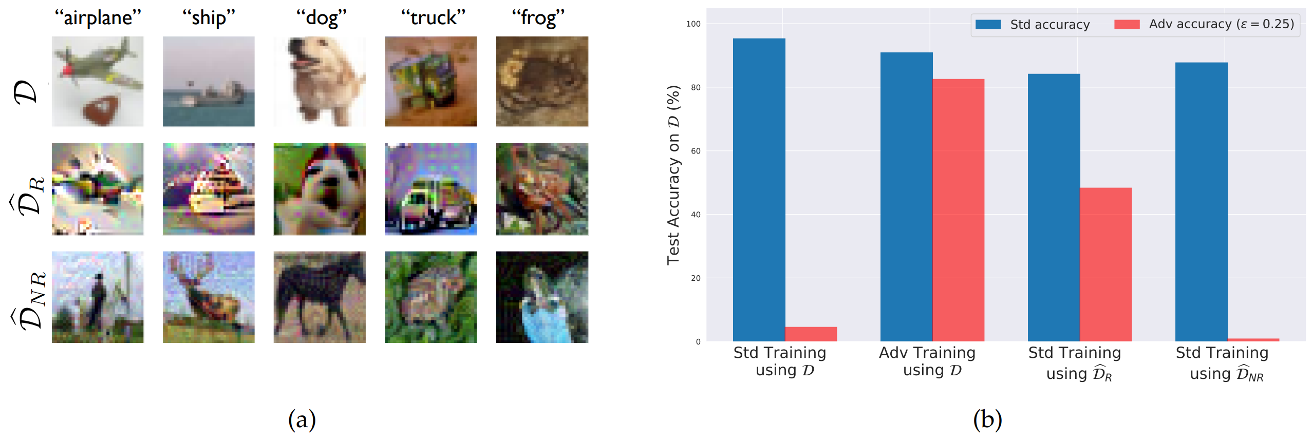
The model trained via standard training on \(\hat{D}_{R}\) (third bar) achieved high standard accuracy on the original test set together with meaningful robust accuracy. In other words, even without performing adversarial training directly, a robust model could be obtained simply by reducing non-robust features in the training data.
Conversely, when standard training was performed on \(\hat{D}_{NR}\) (fourth bar), standard accuracy was preserved but robust accuracy was low. This suggests that a substantial portion of the features used by standard models are non-robust features that are vulnerable to adversarial attacks.
In short, robustness is not solely a property of the learning algorithm; it is also a property of which features are present in the training data.
Generalization Experiment for Non-Robust Features
Objective
The purpose of the second experiment is to verify whether non-robust features are not merely noise but, on their own, generalizable classification information.
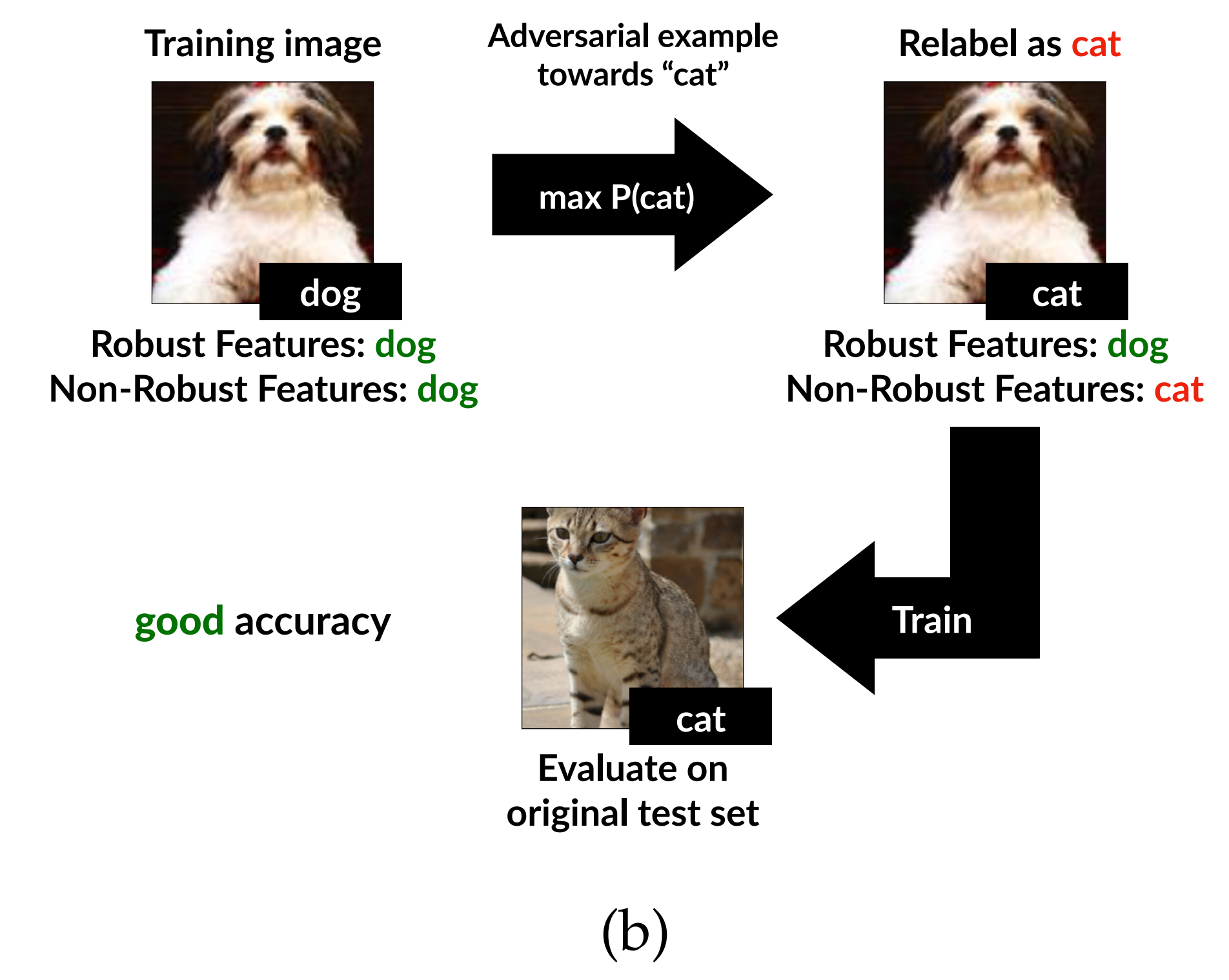
To this end, the authors build a dataset that to a human eye appears mislabeled. Specifically, the visual semantics of each image are kept close to the original class, while only the subtle non-robust features that the model is sensitive to are manipulated to align with a target class.
If a model trained on such a dataset still performs well on the original, normal test set, then non-robust features are not noise that exists by accident only in the training data; they generalize all the way to the test set.
Constructing the Non-Robust Dataset
Given the original image \(x\) and its true label \(y\), the authors first choose a new target class \(t\). They then add a very small perturbation to \(x\) to construct \(x_{adv}\), which appears nearly identical to the original to a human observer but is classified as class \(t\) by a standard model \(C\).
This procedure can be written as the following optimization problem.
\[x_{adv} = \arg\min_{\|x' - x\| \le \epsilon} L_C(x', t)\]That is, under the constraint that the candidate image \(x'\) may differ from \(x\) by at most \(\epsilon\), we find the image whose loss under the standard model \(C\) is smallest when treated as class \(t\).
This is summarized below.
| Data | Visual meaning | Non-robust features the model is sensitive to | Assigned label |
|---|---|---|---|
| \(x\) | \(y\) | \(y\) | \(y\) |
| \(x_{adv}\) | \(y\) | \(t\) | \(t\) |
The authors then attach the label \(t\) to this image and assemble a new training dataset. The meaning of the dataset varies depending on how the target labels are chosen.
| Target label setting | Meaning | Dataset |
|---|---|---|
| Target class chosen at random | Robust features are, on average, uncorrelated with the new label | \(\hat{D}_{rand}\) |
| Mapped from each original class to a fixed different class | Robust features strongly point in the wrong direction | \(\hat{D}_{det}\) |
In \(\hat{D}_{rand}\), the human-visible robust features are essentially uncorrelated with the new labels. In \(\hat{D}_{det}\), by contrast, the robust features more strongly disagree with the new labels. Therefore, if a model trained on \(\hat{D}_{det}\) still generalizes to the original test set, that constitutes strong evidence that the model has truly learned non-robust features.
Results
The paper performs this experiment on CIFAR-10 and on Restricted ImageNet–style datasets. The results are as follows.
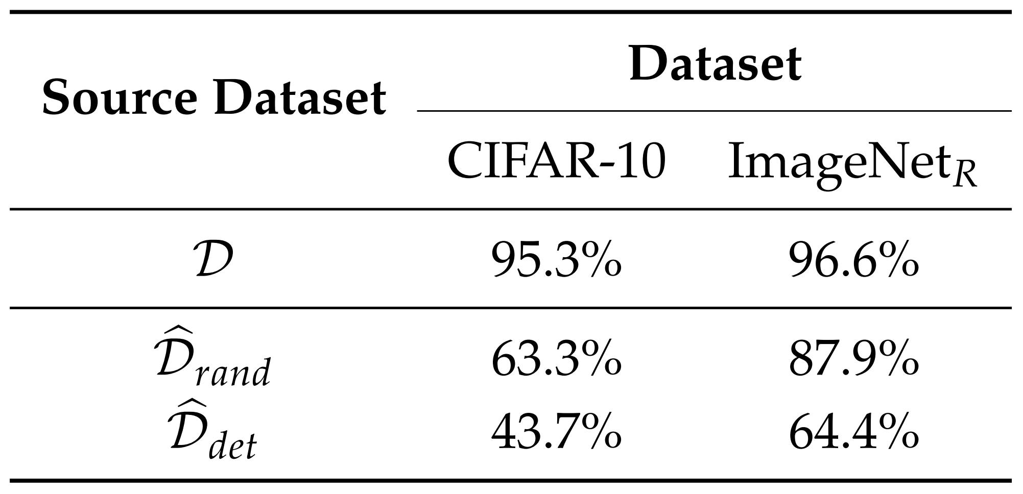
According to the results, although the dataset appears mislabeled to a human, the model learns the non-robust features inside it and achieves substantial accuracy on the original test set. Thus, non-robust features alone are sufficient to obtain standard classification performance. This supports the paper’s claim that adversarial perturbations are not mere errors but the result of manipulating features the model actually uses.
Interpreting Transferability
Motivation
One important property of adversarial examples is transferability: the phenomenon in which an adversarial example crafted for one model also fools another. For example, an adversarial perturbation crafted against ResNet may also affect models with different architectures, such as VGG, DenseNet, or Inception.
It has historically been difficult to clearly explain why this happens. Through the lens of non-robust features proposed in this paper, however, the explanation becomes relatively natural.
Non-Robust Features and Adversarial Transferability
Models trained on the same dataset, even with different architectures, are likely to learn similar predictive information. In particular, if a non-robust feature genuinely exists in the data distribution, multiple models can share it. Thus, a perturbation that manipulates a non-robust feature in one model can also act as an adversarial perturbation against another model — yielding adversarial transferability.
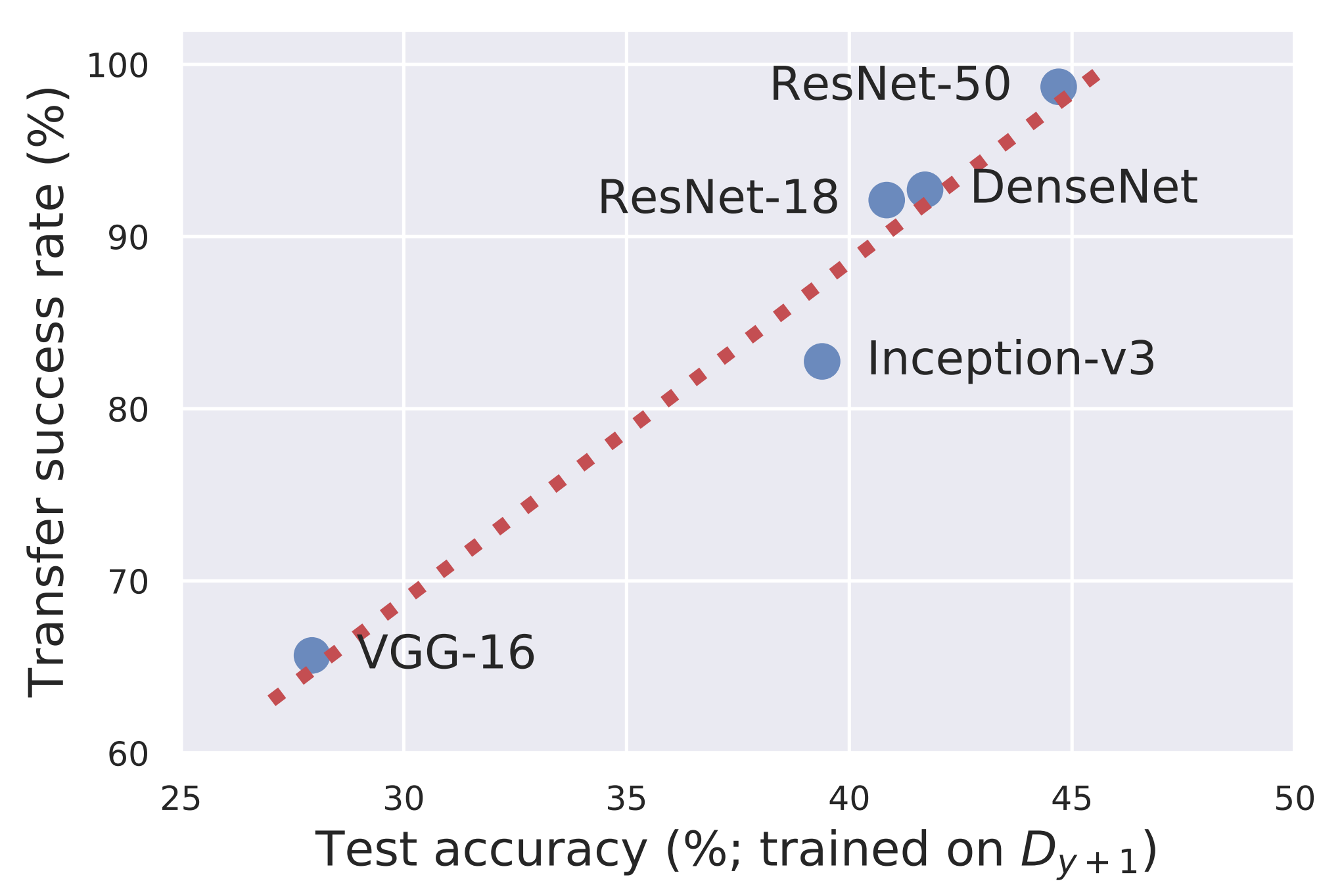
The figure above shows the performance obtained when a non-robust dataset constructed using ResNet-50 is used to train various other architectures. Architectures that better learn from the non-robust dataset also tend to be more easily fooled by adversarial examples crafted against ResNet-50.
This indicates that even different architectures, when trained on the same dataset, can share similar non-robust features, and that perturbations manipulating these features can simultaneously fool multiple models.
Theoretical Analysis
Objective
The previous experiments demonstrate that non-robust features exist in real image datasets and that models learn them. To analyze this in a simpler mathematical setting, the authors consider the problem of classifying two Gaussian distributions.
The Gaussian Classification Problem
The label \(y\) is chosen as either \(+1\) or \(-1\), and the input \(x\) is sampled from a Gaussian distribution whose mean depends on the label.
\[y \sim \{-1, +1\}\] \[x \sim \mathcal{N}(y \cdot \mu^*, \Sigma^*)\]That is, when \(y=+1\), samples are drawn from a distribution centered at \(+\mu^*\), and when \(y=-1\), from a distribution centered at \(-\mu^*\). The model learns the mean \(\mu\) and the covariance \(\Sigma\) in order to determine which class a new input belongs to.
In this model, classification is performed via a likelihood test, which can be written as the following linear decision rule.
\[\hat{y} = \operatorname{sign} \left( x^\top \Sigma^{-1}\mu \right)\]Hence, \(\Sigma\) is not merely a variance estimate; it plays the role of a metric that determines which directions in the input space the model is more sensitive to.
Metric Misalignment
The core of this theoretical analysis is metric misalignment. Here, “metric” refers to the criterion by which distance is measured.
An attacker typically perturbs the input within a human-defined distance budget, such as \(L_2\) or \(L_\infty\). Humans likewise judge that “the image has barely changed” by these criteria. But in the feature space the model has learned, that small change can correspond to a very large semantic change.
In the Gaussian setting, the model parameter \(\Sigma\) induces a data-dependent distance criterion known as the Mahalanobis distance. This distance reflects how the data are spread in different directions.
The relationships are summarized as follows.
| Criterion | Meaning |
|---|---|
| \(L_2\) metric | A human-defined distance in input space |
| Mahalanobis metric | A distance learned by the model from the data distribution |
| Misalignment | A state in which the two criteria disagree |
If, in some direction, an input is moved only a tiny amount in \(L_2\) terms but the change is large in the model’s feature-based metric, that direction is vulnerable to adversarial attacks. The paper identifies this misalignment as the theoretical origin of non-robust features.
The Role of Robust Training
Robust training prevents the model from following only the data-induced metric. It forces the model to also account for the \(L_2\) metric used by the attacker. The paper explains that robust learning produces a hybrid that mixes the data’s inherent metric with the adversary’s metric.
In the paper’s theoretical analysis, the robustly learned covariance takes the following form.
\[\Sigma_{r} = \frac{1}{2}\Sigma^{*} + \frac{1}{\lambda}I + \sqrt{\frac{1}{\lambda}\Sigma^{*} + \frac{1}{4}{\Sigma^{*}}^{2}}\]More important than the precise range of \(\lambda\) is the intuition that robust training mixes a component of the identity matrix \(I\) into the original data covariance \(\Sigma^*\). This can be interpreted as reducing the model’s excessive sensitivity to narrow, fragile directions that are useful only within the data distribution.
Standard training and robust training can therefore be compared as follows.
| Training Method | Distance Criterion |
|---|---|
| Standard training | Uses the metric induced by the data distribution as is |
| Robust training | Compromises between the data metric and the attacker’s metric |
As the perturbation budget \(\epsilon\) available to the attacker grows, the model trusts features along directions that the attacker can easily manipulate less and less. This is visualized as the covariance shifting toward the identity matrix under robust training.
Gradient Interpretability
The paper explains why the gradients of robust models appear more interpretable from the same viewpoint. Standard models, being sensitive to non-robust features, can produce gradients that look like noise to human eyes. Robust models, by relying less on features the attacker can easily manipulate, produce gradients that align more readily with semantically meaningful directions between classes.
In other words, the fact that robust models’ gradients appear more meaningful to humans is not a mere visual coincidence: it is a consequence of the model’s underlying features themselves having shifted in a more robust direction.
Significance and Limitations
Significance
The greatest significance of this paper is that it reinterprets adversarial examples not as a simple model defect but as a natural consequence of the predictive signals in the data combined with the training objective.
In particular, three points stand out.
- Reinterpreting the cause of adversarial examples: Adversarial examples are not the model being fooled by meaningless noise; they can occur precisely because the model has learned genuinely useful non-robust features.
- Explaining the relationship between accuracy and robustness: Non-robust features help standard accuracy. Therefore, removing them or relying on them less can raise robust accuracy but may lower standard accuracy.
- Connecting interpretability and robustness: If the model uses non-robust features that are invisible to humans, post-hoc explanations dressed up to look human-friendly may not be faithful explanations. To improve interpretability, the choice of features the model uses must be controlled during training itself.
Limitations
It is not the case, however, that this paper accounts for every adversarial example purely via non-robust features. The authors themselves show that non-robust features are an important cause of adversarial vulnerability but do not rule out other possible causes.
In addition, robust and non-robust features are not directly observed; they are separated indirectly through the representations used by robust and standard models. Therefore, while the experiments provide very strong evidence, it is hard to claim that every feature in a real-world dataset has been fully decomposed.
Finally, the very notion of “robust” depends on a human-defined perturbation set. For instance, a model that is robust under the \(L_2\) criterion is not necessarily robust to every realistic transformation. Robustness must therefore always be defined with respect to some threat model.
Conclusion
This paper changes the way we view adversarial examples. They had often been understood as a strange malfunction of the model — that is, as bugs. This paper argues that adversarial examples may instead be the result of features the model has actually learned.
The paper’s core message can be summarized in the following three points.
- Non-robust features really exist: Standard image datasets contain subtle features that are barely visible to humans yet helpful for predicting labels.
- Models learn them in pursuit of accuracy: Standard training does not distinguish between robust and non-robust features; it uses any feature that helps accuracy.
- Adversarial attacks manipulate these features: Adversarial perturbations are not meaningless noise but can be understood as flipping the non-robust features the model uses in the opposite direction.
In conclusion, the greatest significance of this work is that it reframes adversarial robustness not as a mere question of defense techniques but as a question of which features we should make our models learn.
Deep learning models do not get fooled because they are stupid. If anything, they exploit the predictive signals in the data too aggressively. The problem is that some of those signals are invisible to humans and highly susceptible to small perturbations.
To build models that are both robust and interpretable, then, it is not enough to bolt on defenses or explanation tools after training. From the very start, training must incorporate appropriate priors and constraints so that the model learns to rely on stable features that humans regard as meaningful.