Paper: Theoretically Principled Trade-off between Robustness and Accuracy
Authors: Hongyang Zhang, Yaodong Yu, Jiantao Jiao, Eric P. Xing, Laurent El Ghaoui, Michael I. Jordan
Venue: International Conference on Machine Learning (ICML 2019)
URL: Theoretically Principled Trade-off between Robustness and Accuracy
Introduction
To build models that are robust to adversarial attacks – attacks that can completely flip a model’s prediction by means of imperceptible adversarial perturbations – prior work has proposed a variety of defense techniques. However, it has been repeatedly observed that the more a model is hardened against adversarial attacks, the more its accuracy on natural examples tends to drop.
This paper investigates this trade-off not as a mere empirical phenomenon but as something rooted in theoretical principles, and proposes TRADES, an optimal defense framework that allows this trade-off to be controlled. The methodology demonstrated its practical effectiveness by ranking first among approximately 2,000 submissions in the NeurIPS 2018 Adversarial Vision Challenge.
Main Contents
An adversarial example is an input designed to flip a model’s prediction by adding a small, human-imperceptible perturbation to a natural example. To quantify how vulnerable a model is to adversarial attacks, the paper defines the robust error as follows.
\[\mathcal{R}_{\text{rob}}(f) := \mathbb{E}_{(\mathbf{X},Y)\sim\mathcal{D}} \mathbf{1}\{\exists X' \in \mathbb{B}(\mathbf{X}, \epsilon) \text{ s.t. } f(X')Y \leq 0\}\]- $f : \mathcal{X} \to \mathbb{R}$ : a binary classifier producing real-valued outputs
- $Y \in {+1, -1}$ : the true label of a sample
- $\mathbb{B}(\mathbf{X}, \epsilon)$ : the $\epsilon$-ball around the natural example $\mathbf{X}$ (the allowed perturbation region)
The expression above measures, for a sample $(X, Y)$ drawn from the natural distribution $\mathcal{D}$, the probability that there exists at least one $X’$ within the allowed perturbation region that causes the model to misclassify. In other words, it adopts a worst-case viewpoint: if even a single attack succeeds within the perturbation region, that sample is counted toward the robust error.
Decomposition of Robust Error
In this paper, the robust error is decomposed into a natural error and a boundary error. For ease of understanding, we present this both in equations and in figures. \(\mathcal{R}_{rob}(f) = \mathcal{R}_{nat}(f) + \mathcal{R}_{bdy}(f)\)
\[\mathcal{R}_{\text{nat}}(f) := \mathbb{E}_{(X,Y)\sim\mathcal{D}} \mathbf{1}\{f(X)Y \leq 0\} \\ \mathcal{R}_{\text{bdy}}(f) := \mathbb{E}_{(X,Y)\sim\mathcal{D}} \mathbf{1}\{X \in \mathbb{B}(\text{DB}(f), \epsilon),\ f(X)Y > 0\}\]- $\mathcal{R}_{nat}$ : the error of the model misclassifying the natural example itself (natural error)
- $\mathcal{R}_{bdy}$ : the error in which the natural example is classified correctly, but a perturbation that crosses the decision boundary exists within the $\epsilon$-ball (boundary error)
The decomposition above implies that, in order to improve a model’s robustness, it is not enough to merely improve classification performance; the decision boundary must also be pushed far away from the data to reduce the boundary error.
Intuitively, this can be understood as follows. Around each sample lies an allowed perturbation region (the $\epsilon$-ball). If the decision boundary does not cut through this $\epsilon$-ball, the sample enjoys both natural and robust accuracy. Conversely, when the $\epsilon$-ball crosses the decision boundary, even a tiny perturbation can cause misclassification, which corresponds to the boundary error ($\mathcal{R}_{bdy}$). By using adversarial training to push the decision boundary away from the data, we can reduce the boundary error for samples near the boundary.
Surrogate Loss Functions
To learn a model that adjusts the decision boundary, we need to compute the gradient of a loss function. However, a loss that returns +1 on errors and 0 on correct predictions is discrete in value and therefore not differentiable. Hence, the paper performs optimization using a surrogate loss $\phi$ in place of the 0-1 loss.
A natural question is then: “Does minimizing the surrogate loss truly correspond to minimizing the 0-1 loss?” To guarantee this, the authors introduce the condition that “the surrogate loss function $\phi$ is classification-calibrated.” This condition ensures that the direction of minimizing the surrogate loss $\phi$ ultimately aligns with the decision direction of the Bayes optimal classifier, which minimizes the 0-1 loss.
To make this more concrete, let us look at how the loss function is defined in a binary classification setting.
Suppose we have a function $f$ and a data distribution $(x, y) \sim \mathcal{D}$ with $y \in {-1, +1}$, and let $f(x) = \alpha$. Consider a classifier that makes the following predictions:
- If $\alpha > 0$, predict $y = +1$
- If $\alpha < 0$, predict $y = -1$
Then $\alpha y > 0$ corresponds to a correct prediction, and $\alpha y < 0$ to an incorrect one. A good loss function should return small values when the prediction is correct and large values when it is wrong. In other words, the sign and magnitude of $\alpha y$ are the key information determining the loss. The function that computes this loss is $\phi(\alpha y)$.
When the function value is $\alpha$, let
- $\eta$ : the probability that the true label of this $\alpha$ is $y = +1$
- $1 - \eta$ : the probability that the true label of this $\alpha$ is $y = -1$.
Once $\eta$ is known, the optimal classifier is automatically determined.
- $\eta > 0.5 \rightarrow$ since $y = +1$ is more likely, the classifier should output $\alpha > 0$
- $\eta < 0.5 \rightarrow$ since $y = -1$ is more likely, the classifier should output $\alpha < 0$
The optimal classifier that, at each $x$, picks the more likely class in this manner is called the Bayes optimal classifier.
Let the corresponding expected loss be $C_\eta(\alpha)$, and define $H(\eta)$ as the minimum value of $C_\eta(\alpha)$ when $\alpha$ is varied over the entire real line. Formally:
\[H(\eta) := \inf_{\alpha \in \mathbb{R}} C_\eta(\alpha) := \inf_{\alpha \in \mathbb{R}} \left( \eta\phi(\alpha) + (1-\eta)\phi(-\alpha) \right)\]Whereas $H(\eta)$ is the minimum of $C_\eta(\alpha)$ when $\alpha$ is freely chosen, $H^-(\eta)$ is defined as the minimum when $\alpha$ is forced to point in the direction opposite to the Bayes optimal one:
\[H^-(\eta) := \inf_{\alpha:\,(2\eta-1)\alpha \leq 0} C_\eta(\alpha)\]Since $H^-(\eta)$ is the minimum loss attained when the classifier is forced to produce the wrong answer, $H^-(\eta) \geq H(\eta)$ always holds. If, in addition, $H^-(\eta) > H(\eta)$ holds for every $\eta \neq 1/2$, then $\phi$ is called a classification-calibrated loss. Moreover, the larger $H^-(\eta) - H(\eta)$ is, the more strongly the surrogate loss $\phi$ pushes the classifier toward the Bayes optimal direction. The function that quantifies this is $\tilde{\psi}$.
\[\tilde{\psi}(\theta) = H^-\!\left(\frac{1+\theta}{2}\right) - H\!\left(\frac{1+\theta}{2}\right)\]However, $\tilde{\psi}$ itself is not guaranteed to be mathematically convex, so to develop the upper- and lower-bound proofs that follow, a new function $\psi = \tilde{\psi}^{}$ is defined by applying the bi-conjugate operation. The resulting $\psi(\theta)$ is the **largest convex lower bound that can be drawn beneath the original function $\tilde{\psi}$, and inherits the properties of a convex function.
By adopting a surrogate loss $\phi$ that satisfies this classification-calibration condition, the authors are able to establish, via the $\psi$ transform, a precise mathematical relationship between the surrogate loss risk and the true 0-1-loss-based error.
Tightness via Upper and Lower Bounds
What this paper aims to minimize is the gap between the model’s robust error and the optimal natural error, expressible as $\mathcal{R}{rob}(f) - \mathcal{R}^*{nat}$.
Furthermore, prior work (Bartlett et al., 2006) showed that, when the surrogate loss function $\phi$ satisfies the classification-calibration condition, the following inequality holds:
\[\mathcal{R}_{nat}(f) - \mathcal{R}^*_{nat} \leq \psi^{-1}(\mathcal{R}_\phi(f) - \mathcal{R}^*_\phi)\]Combining this with the definitions introduced earlier in the paper yields the following upper bound on $\mathcal{R}{rob}(f) - \mathcal{R}^*{nat}$:
\[\mathcal{R}_{rob}(f) - \mathcal{R}^*_{nat} \leq \psi^{-1}(\mathcal{R}_\phi(f) - \mathcal{R}^*_\phi) + \mathcal{R}_{bdy}(f)\] \[\mathcal{R}_{rob}(f) - \mathcal{R}^*_{nat} \leq \psi^{-1}(\mathcal{R}_\phi(f) - \mathcal{R}^*_\phi) + \Pr[X \in \mathbb{B}(\text{DB}(f), \epsilon), f(X)Y > 0]\leq \psi^{-1}(\mathcal{R}_\phi(f) - \mathcal{R}^*_\phi) + \mathbb{E} \max_{X' \in \mathbb{B}(X, \epsilon)} \phi(f(X')f(X)/\lambda)\]This inequality mathematically guarantees that “if we reduce the surrogate loss expression that we can actually compute, the true adversarial error – which we cannot directly compute – is also pressed down by this upper bound.”
To verify how tight the upper bound formula is, the authors then prove a corresponding lower bound in the opposite direction.
The authors show that, even under extreme worst-case assumptions, the surrogate-loss expression we compute can never fall below the upper bound formula derived above.
The experiments that validate this tightness are described in detail in the experiments section.
TRADES Algorithm
So far, we have seen how the upper bound on the adversarial error was mathematically established. The authors translate this theoretical upper bound into the following optimization objective.
Building on the right-hand side of the upper bound from the theoretical part (the surrogate loss plus the differentiable boundary error), the authors propose the following final training objective:
\[\min_f \mathbb{E}\left\{ \underbrace{\phi(f(X)Y)}_{\text{for accuracy}} + \underbrace{\max_{X' \in \mathbb{B}(X,\epsilon)} \phi(f(X)f(X')/\lambda)}_{\text{regularization for robustness}} \right\}\]For the sake of implementation simplicity, the cumbersome inverse function \(ψ^{−1}\) is dropped, and a parameter \(λ\) is used instead to balance the two terms.
-
First term: minimizes the discrepancy between the model’s prediction \(f(X)\) and the true label \(Y\), thereby maximizing natural accuracy.
-
Second term: forces the output distributions on the original input \(X\) and the adversarially perturbed input \(X′\) to remain close, acting as a regularizer that pushes the decision boundary away from the data.
The authors further extend the binary-classification-based theoretical framework developed so far to a real-world deep learning setting, namely multi-class image classification. To this end, they replace the surrogate loss \(\phi\) above with the cross-entropy loss \(L(\cdot,\cdot)\), a multiclass calibrated loss, and implement TRADES with the following final formulation. \(\min_{f} \mathbb{E} \left\{ \mathcal{L}(f(\mathbf{X}), \mathbf{Y}) + \max_{\mathbf{X}' \in B(\mathbf{X}, \epsilon)} \mathcal{L}(f(\mathbf{X}), f(\mathbf{X}'))/\lambda \right\}\)
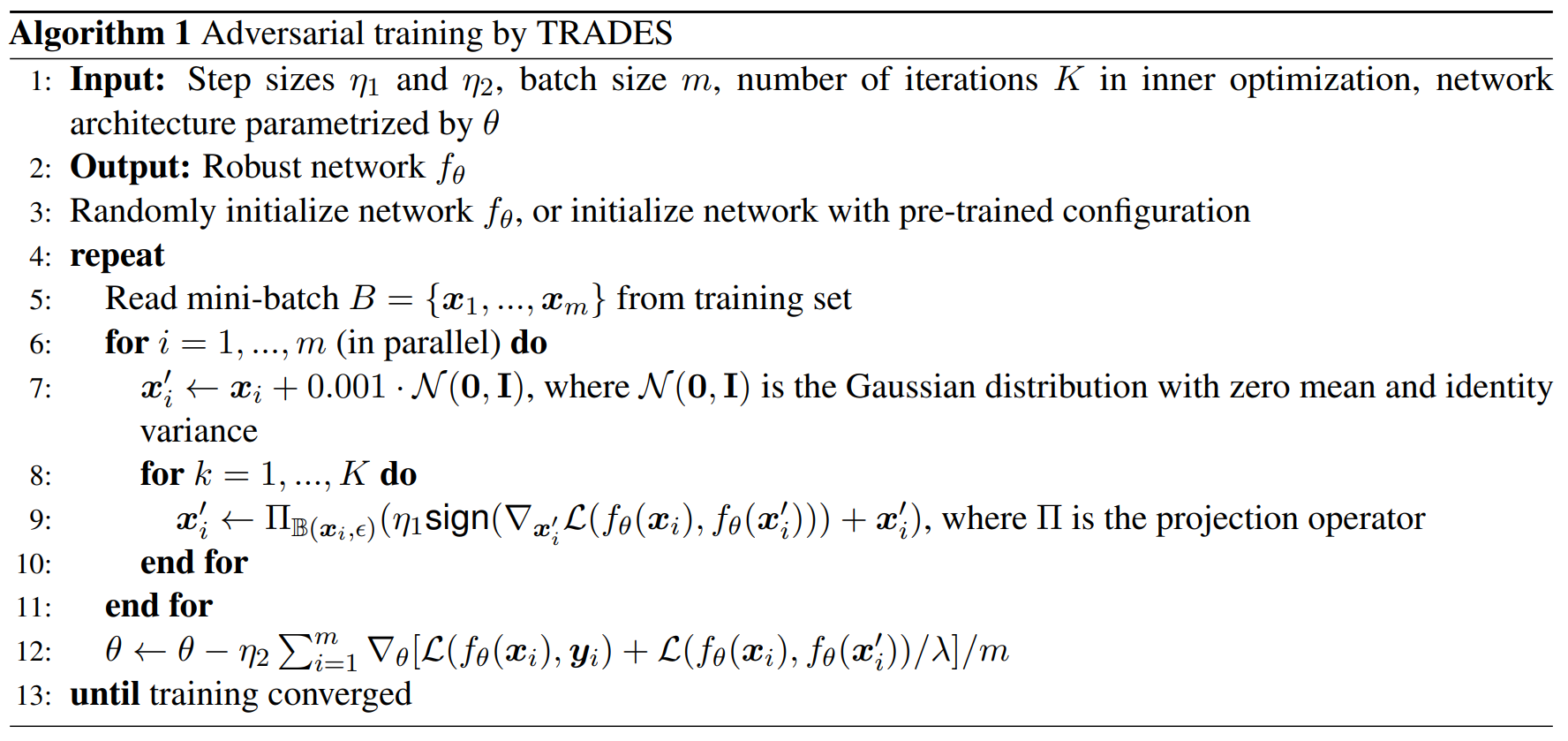
The key lines of the algorithm above are lines 7, 9, and 12.
-
line 7: For each sample \(x_i\), a small Gaussian noise is added to initialize \(x'_i\). This is because the inner objective \(g(x')=\mathcal{L}(f_\theta(x_i), f_\theta(x'))\) attains its minimum and has zero gradient at \(x'=x_i\), so a random start is used to prevent the optimization from getting stuck right from the beginning.
-
line 9: With the parameters \(\theta\) fixed, \(x'_i\) is updated by projected gradient ascent for \(K\) steps, approximately solving \(\max_{x'_i \in B(x_i,\epsilon)} \mathcal{L}(f_\theta(x_i), f_\theta(x'_i))\). The crucial point is that the loss to be increased here is not the standard adversarial-training loss \(\mathcal{L}(f_\theta(x'_i), y_i)\) but rather \(\mathcal{L}(f_\theta(x_i), f_\theta(x'_i))\), which measures the discrepancy between the predictions on the original and perturbed inputs. At every step, \(x'_i\) is moved in the direction that increases this loss and then projected so that it always remains inside \(B(x_i,\epsilon)\).
-
line 12: Using the \(x'_i\) obtained in line 9, the model parameters \(\theta\) are updated. The first term \(\mathcal{L}(f_\theta(x_i), y_i)\) keeps the accuracy on clean samples, while the second term \(\mathcal{L}(f_\theta(x_i), f_\theta(x'_i))/\lambda\) prevents the prediction from changing abruptly under nearby perturbations, thereby pushing the decision boundary away from the data. Hence \(\lambda\) controls the balance between natural accuracy and robustness.
Experiments
The paper validates (1) the tightness of the theoretical upper bound, (2) the robustness-accuracy trade-off induced by the regularization coefficient \(\lambda\), (3) the actual defense performance under various attacks, and (4) the effectiveness in a real competition setting through experiments.
Tightness Verification
The authors verify how tight their proposed upper bound actually is. That is, they examine, against worst-case adversarial examples, how close the left-hand side \(\Delta_{\mathrm{LHS}}\) and the right-hand side (the upper bound) \(\Delta_{\mathrm{RHS}}\) of the upper-bound inequality are. \(\Delta_{\mathrm{LHS}} = \mathcal{R}_{\mathrm{rob}}(f) - \mathcal{R}^*_{\mathrm{nat}}.\)
\[\Delta_{\text{RHS}} = (\mathcal{R}_{\phi}(f) - \mathcal{R}_{\phi}^{*}) + \mathbb{E} \max_{X' \in \mathcal{B}(X, \epsilon)} \phi((f(\mathbf{X}')f(\mathbf{X})/\lambda)).\]For this purpose, the authors construct a binary classification problem on MNIST using only the digits 1 and 3, and use a CNN consisting of 2 convolutional layers and 2 fully-connected layers. As the surrogate loss they use the hinge loss, in which case \(\psi(\theta)=\theta\), so the right-hand side simplifies as above. In the experiments, the perturbation budget is set to \(\epsilon = 0.1\) and the inner maximization of TRADES is performed with \(K = 20\) steps. Furthermore, since the distribution \(\mathcal{D}\) cannot be known directly, the expectations are approximated using the test set, and the worst-case perturbed sample \(X'\) required for the second term of \(\Delta_{\mathrm{RHS}}\) is approximated using a 20-step FGSMk (PGD) attack.
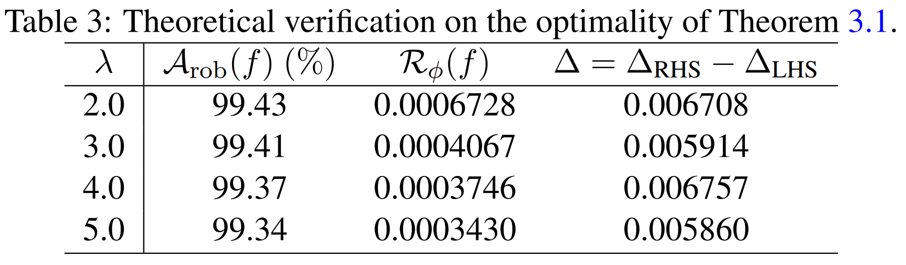
As a result, in the table above, \(\Delta = \Delta_{RHS} - \Delta_{LHS}\) is on the order of approximately 0.0059-0.0068, which is very small. In other words, the theoretically derived upper bound does not loosely envelop the actual robust error; experimentally it tracks it quite accurately.
Effect of Regularization Coefficient \(\lambda\)
The next experiment moves on to multi-class classification, applying cross-entropy-based TRADES on MNIST and CIFAR10. A small CNN is used on MNIST and ResNet-18 on CIFAR10, and on both datasets the changes in natural accuracy \(A_{nat}\) and robust accuracy \(A_{rob}\) are observed as \(\frac{1}{\lambda}\) is varied.
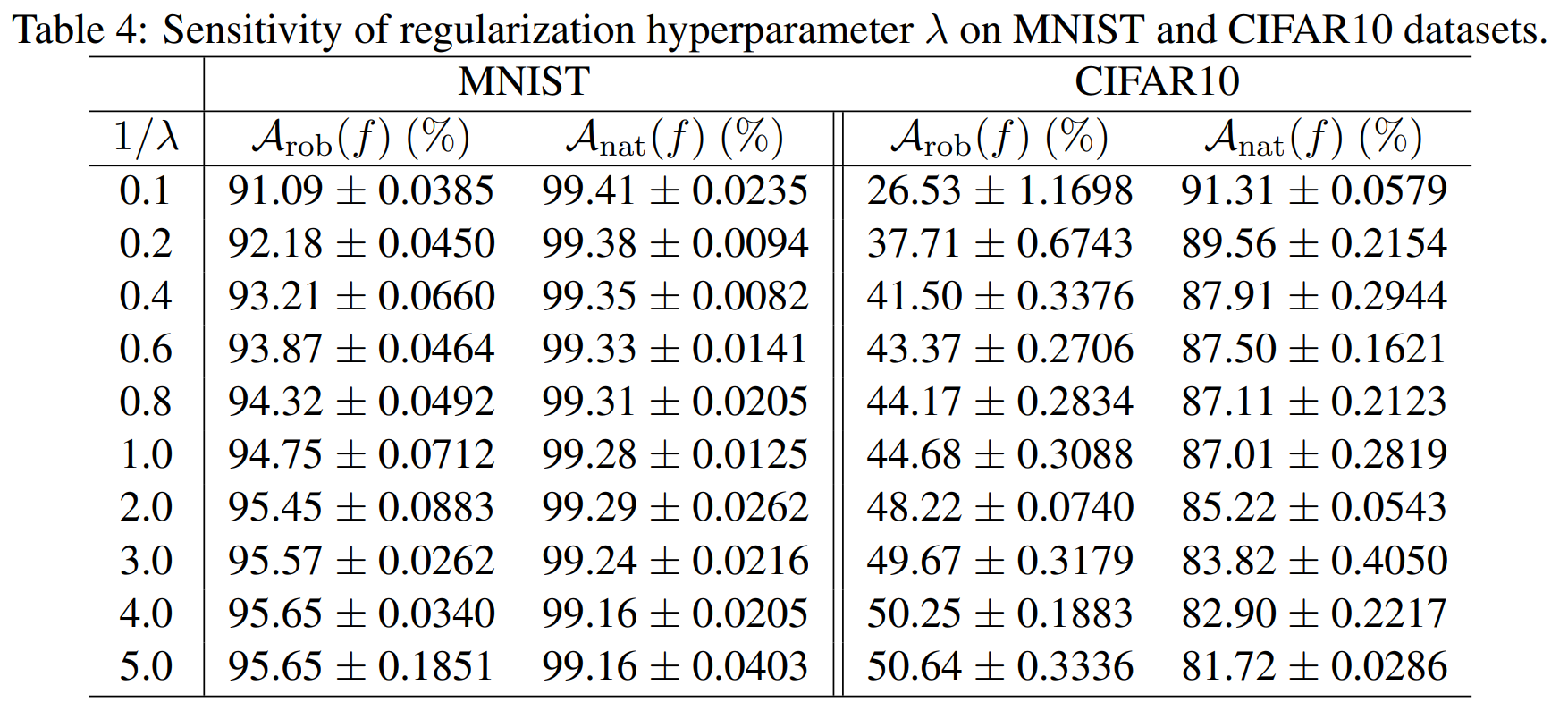
The table above conveys the central message of TRADES directly. As \(\frac{1}{\lambda}\) increases, the regularization becomes stronger, the decision boundary moves farther from the data, and at the cost of a slight drop in natural accuracy the robust accuracy rises.
Since the MNIST classification task is easier than CIFAR10, the drop in natural accuracy is relatively small. The authors thus argue that the trade-off between robustness and accuracy is observed not only in theory but also in real datasets.
Defense Performance Across Attacks
The paper compares TRADES with existing defense techniques under both white-box and black-box attacks.
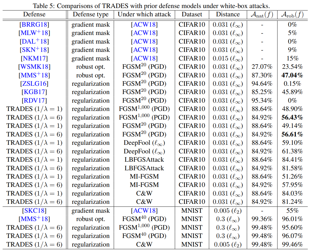
The table above shows the defense results under white-box attacks. The white-box attack experiments use different models and attack settings depending on the dataset. On MNIST, the CNN architecture from [CW17] is used, with a perturbation budget of \(\epsilon=0.3\), step size \(\eta_1=0.01\), and \(K=40\) inner iterations. On CIFAR10, the same WRN-34-10 as in Madry et al. [MMS+18] is used, with \(\epsilon=0.031\), \(\eta_1=0.007\), and \(K=10\).
In this setting, TRADES achieves higher robust accuracy than the existing defense techniques. For instance, under the PGD 20-step attack on CIFAR10, it records 56.61%, surpassing the 47.04% of the Madry model, and it also consistently outperforms on other white-box attacks such as DeepFool, MI-FGSM, and C\&W.
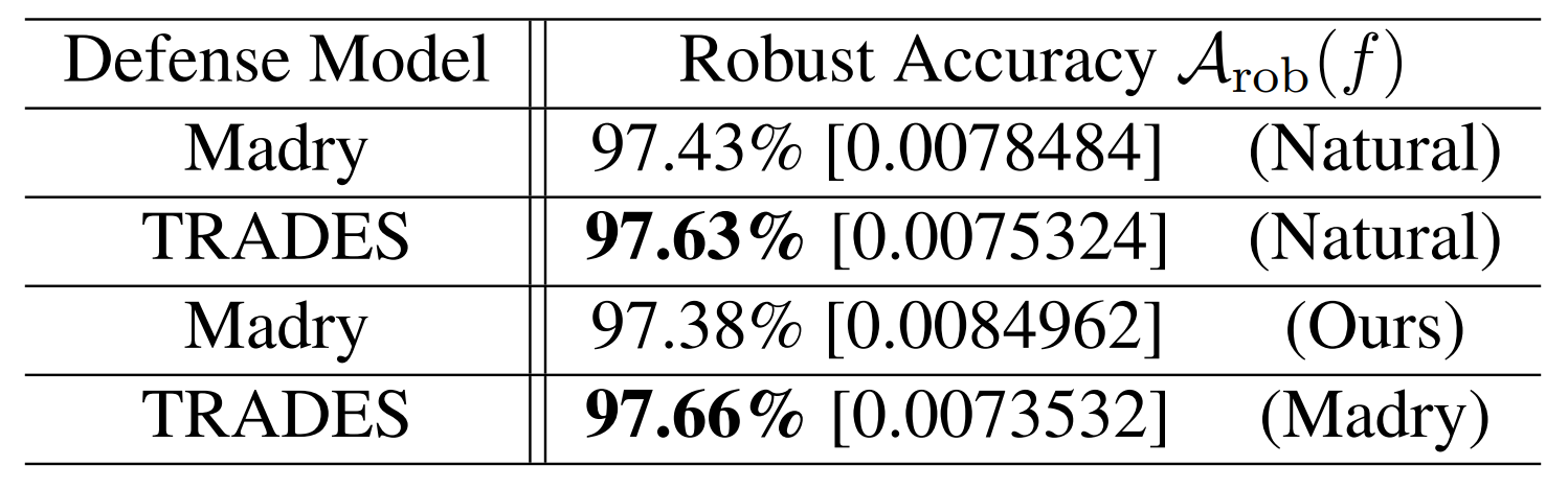
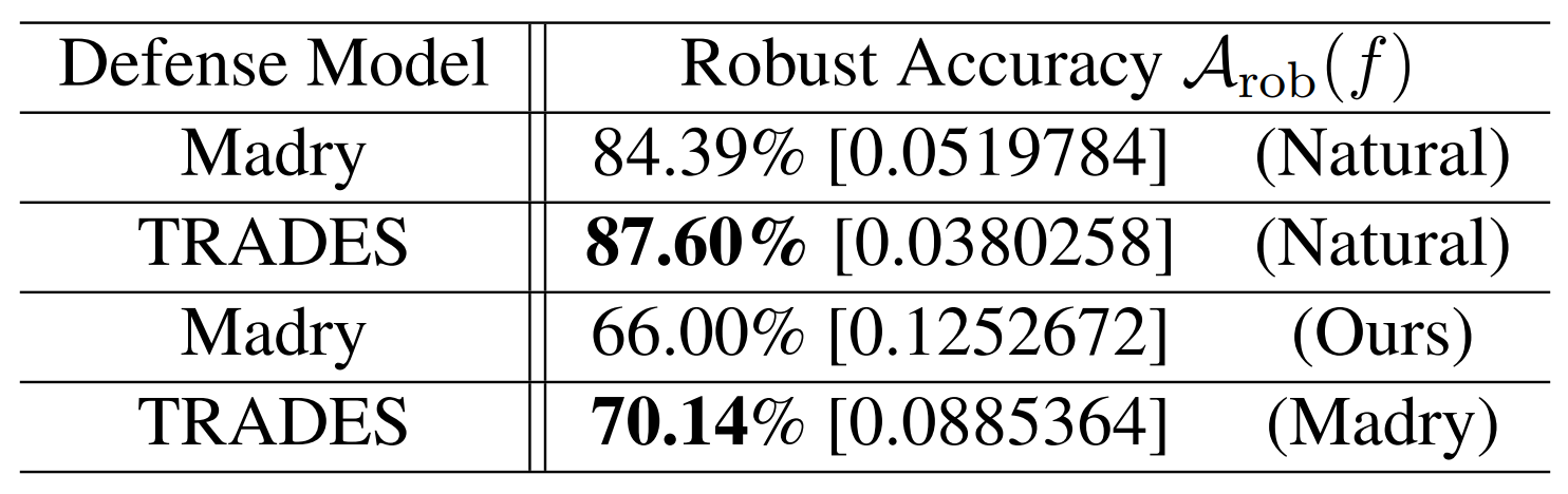
The two tables above show the defense results under black-box attacks. The contents inside parentheses indicate the source model used to generate the adversarial examples, while the contents inside square brackets indicate the average loss of the defense model when fed those examples.
Experimentally, TRADES records higher robust accuracy than the Madry model under transfer attacks on both MNIST and CIFAR10. For example, when a Natural model is used as the source model, on MNIST TRADES achieves 97.63% versus 97.43% for Madry, and on CIFAR10 in the same setting TRADES achieves 87.60% versus 84.39% for Madry.
In short, TRADES is not only strong against white-box attacks but also exhibits comparatively stable defense performance against black-box attacks.
Conclusion
This paper theoretically explains the trade-off between adversarial robustness and natural accuracy, and proposes TRADES, a new adversarial-training objective that allows this trade-off to be precisely controlled.
The authors decompose the robust error into a natural error and a boundary error, and use a classification-calibrated surrogate loss to derive the mathematically tightest upper bound on the robust error.
Through experiments, they further demonstrate that the regularization coefficient \(\lambda\) indeed controls the balance between robustness and accuracy, and confirm that TRADES outperforms existing defense techniques across a variety of attack settings.
In conclusion, the central contribution of this paper is to elevate the robustness-accuracy trade-off from a mere empirical phenomenon to an algorithmic framework grounded in mathematical principles (Theoretically Principled).